A rieg is a commutative semiring equipped with exponentiation satisfying the usual exponent laws, including x0=1 and hence 00=1. This project studies the structure itself and the examples it connects.
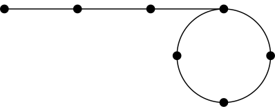
For finite-valued presheaves, essentially finite slices give a sufficient condition for a topos. A partial answer proposes an exact criterion stated in terms of finite presheaves. The right Kan extension approach is absorbed into that note, with the coreflection X↦Xfin onto locally finite presheaves as its comonad.
The next step is concrete: give a criterion for finite presheaf topoi in terms of the indexing category alone.
Work in progress. The Introduction is incomplete.
NOTES ON RIEG THEORY: SEMIRING WITH EXPONENTIALS IN LOGIC, PROFINITE
ARITHMETIC, ENUMERATIVE COMBINATORICS, AND CATEGORY THEORY
RYUYA HORA
Abstract.In this paper, we introduce the notion of a rieg, that is, a semiring equipped with a binary operation
called exponentiation, and present its basic theory along with numerous examples. We begin by reviewing the
classification of quotient riegs over given by Burris and Lee. Then, through concrete examples, we propose how riegs can appear in (pro)finite arithmetic,
category theory, enumerative combinatorics, and logic. Typical examples of a rieg include the rieg of natural numbers,
the five cyclic models (and ),
other quotient riegs of (modulo arithmetic with exponentials), the canonical profinite rieg ,
the topological rieg of -adic
natural numbers (which does not work for the -adic
natural numbers ),
the cardinal arithmetic like ,
the rieg of truth values with ,
Heyting algebras including the set of open subsets of a topological space ,
the rieg of finite directed graphs, the Burnside rieg of a finite group, the rieg of rooted trees, the rieg of isomorphism
classes of finite groups, and other decategorified topoi.
Key words and phrases. Semiring, rig, exponential, profinite set, Tarski highschool problem, objective number theory,
cartesian closed category, topos, Burnside rig, Heyting algebra, equational theory.
1. Introduction
The aim of the present paper is to popularise an algebraic structure, which we will call riegs,
by providing several theorems and examples. As a rig defined as a “ring without negatives”
([Sch90]) a rieg is a “rig with exponentials.” In other words, a rieg is a ring-like structure that has
and a binary
operation
(Definition 2.2.1). The prototypical example of a rieg is the rieg of natural numbers.
Of course, the idea of considering ring-like structures with exponentials is not new.
To the best of the author’s knowledge, the field in which rigs with (binary) exponentiation have been most actively
studied is (finite) model theory. The Tarski High School problem concerns the theory of the positive integers with addition,
multiplication, and exponentiation. Even after this problem was resolved, research on small models continued to progress.
The story until 2005 is summarized in [BY05].
Acknowledgement. The author would like to thank his supervisor Ryu Hasegawa for helpful discussions and suggestions.
He was supported by JSPS KAKENHI Grant Number JP24KJ0837 and FoPM, WINGS Program, the University of Tokyo.
He is also grateful to Ivan Di Liberti for pointing out Remark 2.3.3.
Survey.
One can see the idea of an algebra of structures, with exponential in [Bir42].
Wilkie gives a solution to Tarski’s high school algebra problem, circulated as a preprint and published
in 2000 [Wil00].
[BL92] (and its summary [BL93]) give what we call the Burris-Lee theorem
Schanuel publishes papers on objective number theory [Sch00a][Sch00b]
Fiore, Cosmo, and Balat give a type-theoretic view on this structure, with
[FDB06].
Notation 1.0.1. We adopt the following notations:
denotes the set of all non-negative integers. Sometimes, we regard it as a poset with the natural ordering.
denotes the set of all positive integers. We may regard it as a poset with the divisibility order.
2. Riegs
2.1. Preliminaries: rigs.
Since our theory of riegs is based on the theory of rigs
(
semirings), we start by recalling the notion of rigs. (The word “rig” comes from “ring without negatives” [Sch90].) We only
need the definition and a few examples.
Definition 2.1.1 (Rig). A (possibly non-commutative) rig is a set
equipped
with
two constants (
nullary operations)
and
two binary operations,
such that the following equations hold for all :
(1)
,
(2)
,
(3)
,
(4)
,
(5)
,
(6)
,
(7)
,
(8)
,
(9)
,
and
(10)
.
If satisfies
an additional equation
(11)
,
we call it a commutative rig. A rig homomorphism is a function that preserves the four operations
. The category of rigs and rig
homomorphisms is denoted by .
For the sake of simplicity, we may write
for . Let
us provide three examples, each of which plays a specific role in what follows.
Example 2.1.2 (Rings). Of course, every ring is a rig; the theory of rigs is obtained from that of rings by dropping
the axiom that every element has an additive inverse. However, rings will play only a marginal role in this paper:
we will see that the only rieg whose underlying rig is a ring is the degenerate one (Proposition 2.3.2).
Example 2.1.3 (Rig of natural numbers). The rig of natural numbers (with the usual addition and multiplication)
is the initial object of the category .
Its quotients will be the main subject of Section 3.
Example 2.1.4 (Rig of endohomomorphisms on a commutative monoid). For a commutative monoid
, the set of monoid
endohomomorphisms
admits a rig structure as follows:
The element
is the constant function to the neutral element .
The element
is the identity function .
The sum
of two elements
is given by .
(Here, we use the commutativity of .)
The product
of two elements
is given by the composite .
For the additive monoid , the
rig is isomorphic to the
rig of natural numbers .
A rig of endohomomorphisms is, however, typically non-commutative; for the additive group
, the rig
is isomorphic
to the ring of
matrices
over ,
which is not commutative. This is the example that we will use to define riegs (Definition 2.2.1).
2.2. Definition. This subsection aims to introduce the notion of riegs. Although it is possible to define riegs by familiar
but numerous equations (Proposition 2.2.2), we adopt another definition, which turns out to be surprisingly simple. Note
that in
the definition below is the rig explained in Example 2.1.4 obtained from the multiplicative commutative monoid
.
Definition 2.2.1 (Rieg). A rieg is a commutative rig
equipped with a rig homomorphism .
At first glance, this definition may not seem to have anything to do with exponents.
So let us unpack the definition into a sequence of equalities. The rig homomorphism
sends an
element
to a (commutative) monoid homomorphism, which will be denoted by
The condition that
is a monoid homomorphism is equivalent to the familiar equations
,
and
.
For the function to be a rig
homomorphism, it must preserve ,
,
, and
.
Preservation of each operation corresponds to the equation listed in Table 1.
Preserved rig structure
The required equation
Table 1. Four of the rieg equations
Summarising the above observations, we obtain an equational definition of the notion of riegs. While it is longer than
Definition 2.2.1, it consists only of familiar conditions.
Proposition 2.2.2 (Equational definition of riegs).The definition of riegs (Definition 2.2.1) can be rephrased by the five
operations:
two constants (nullary operations), ,
and
three binary operations, ,
and fourteen equations:
(1)
(2)
(3)
(4)
(5)
(6)
(7)
(8)
(9)
(10)
.
(11)
(12)
(13)
(14)
,
where denotes ,
and denotes as usual.
If we forget the constant ,
these are exactly the eleven “high school identities” of Tarski [BY05]. The other three equations,
,
, and
, are the ones
that involve .
Remark 2.2.3. As a special case of the equation ,
we have .
This convention will be repeatedly interpreted in many ways in this paper.
From this equational (or algebraic) definition, we can define the notion of rieg homomorphisms in the usual
way.
Definition 2.2.4.A rieg homomorphism is a function that preserves all (five) operations .
We write
for the category of riegs.
As we will see numerous examples later, for now, we introduce only two trivial (but important!) examples of riegs: the
initial object and the terminal object in the category of riegs.
Example 2.2.5 (The initial rieg: natural numbers). The set of all natural numbers
equipped with
the usual zero ,
one , addition
, multiplication
, and exponentiation
, forms the rieg of
natural numbers .
Here are a few remarks about this example:
This rieg
is an initial object in the category .
Indeed, for a rieg ,
the unique rig homomorphism
automatically preserves :
for ,
the equations ,
,
and
give ,
where both products have
factors.
This is the unique rieg structure on the rig of natural numbers, since
is the initial rig (Example 2.1.3) and a rieg structure is given by a rig homomorphism .
Example 2.2.6 (The degenerate rieg). A singleton
admits exactly one rieg structure, which we call the degenerate rieg .
The degenerate rieg is a terminal object of the category .
2.3. Digression: Why rigs, not rings?. The reader may wonder: why do we develop our theory using rigs, even though
rings are so famous and successful? There are several possible answers, but perhaps the simplest is that subtraction and
exponentiation are fundamentally incompatible—if we have subtraction, then we have to give a meaning to
!
Claim 2.3.1.If a rieg contains an additive inverse of ,
then it is degenerate, that is, (cf. Example 2.2.6).
Proof.We have the equation
This implies that every element
is equal to ,
since .
□
Proposition 2.3.2 (No rieg is a ring).If a rieg is a ring, then it is degenerate, that is, .
Proof.A ring contains an additive inverse of ,
so Claim 2.3.1 applies. □
Remark 2.3.3. A similar problem appears for division, and there we have a solution. A meadow is a commutative
ring with a total inverse operation, and its axioms imply
[BHT09]. So we may hope to do the same thing here, that is, to choose a value of .
This does not work. Whatever the value of
is, we have ,
and the proof of Claim 2.3.1 still gives .
For example, exponentiation can be defined on the rig
, but it is impossible
on the ring
(Proposition 2.3.2). To the best of the author’s understanding, one reason why exponential structures—despite being
present in many mathematical objects—have not received the attention they perhaps deserve is that the
process of decategorification often involves introducing formal subtraction. For example, the ring of integers
is obtained by introducing
a formal subtraction to ,
which inherently admits the exponential structure of the cartesian closed category
(Section 4). This subtraction does help clarify theories (sometimes by reducing the amount of information), but at the same
time, it forces us to entirely forget the exponential structure.
3. Example 1: Riegs in finite and profinite arithmetic
3.1. Rieg theoretic phenomena. Before delving into the technical details, let us first take a look at a few phenomena
that will be studied in the rest of this section.
3.1.1. Phenomenon 1: modular arithmetic with exponentials. Let us consider the following high school level problem from
elementary number theory, which involves exponentiation.
Puzzle 3.1.1.Find all pairs of natural numbers
such that
Answer.Consider the equation modulo .
If , the
equation is simplified to
However, since the quadratic residues modulo are ,,
and ,
it is impossible. Therefore, we only need to check ,,
and .
We conclude that the only solution is .
In this example, when considering exponentiation modulo
, we have to set aside the “first
exceptions”, namely the three numbers .
3.1.2. Phenomenon 2: Profinite dynamical systems with exponentials.
Let us consider the following puzzle.
Puzzle 3.1.2 (A puzzle provided by J.Koizumi).Find a four-digit natural number
such that the last four digits of
are equal to .
There is a surprisingly simple way to obtain the solution — namely, iteration! First, take an arbitrary natural number
, say
. Then, repeatedly replace
by the last four digits of
1.
We obtain an answer .
Answer.is the only answer.
Then, it is natural to ask whether we can go farther:
Question 3.1.3.Is there an infinite sequence of decimal digits
such that, for every integer ,
the truncation satisfies the congruence
Remark 3.1.4 (Attribution). The affirmative answer is not new. It is a special case of a theorem of Jiménez Urroz
and Yebra [JY09, Theorem 3]: for every valid base
(an integer such that
for every prime
and every prime )
and every integer
not divisible by the squarefree part of ,
there is a unique such digit sequence for the congruences
for all sufficiently large .
The base
is valid, and our digit sequence is recorded as [OEIa], known there as the final digits of Graham’s number; the
truncations displayed in Figure 1 form [OEIb]. What rieg theory adds is not the statement but a conceptual proof:
the sequence is the unique fixed point of the contraction
(Proposition 3.3.12).
This phenomenon is reminiscent of -adic
integers. Indeed, the stabilization of the digits of an iterated exponential (or tower) modulo a fixed number is
classically known, and is even used as a computational tool [Hit20]. However, in this case, the exponential
operation is involved not only as an iteration of a fixed function but as a binary operation on the number system
itself.
In this section, we will construct profinite systems of numbers, which can be regarded as
-adic
number systems with exponentials. Using that structure, we will be able to answer the above question easily.
The rough sketch of our proof is as follows:
Answer (Rough sketch).
In a topological rieg (Definition 3.3.6), we can take the limit of the sequence
By the continuity of ,
we have .
Furthermore, the fixed point
turns out to be unique, which explains why the iteration in the above puzzle reaches the same answer regardless of the starting value:
we will later regard
as a contraction with respect to a natural metric and apply the Banach fixed-point theorem (Proposition 3.3.12).
3.1.3. Phenomenon 3: Well-defined modulo exponentials. Let us conclude this subsection by introducing the fact that first
attracted the author to riegs. As far as the author knows, it was originally proven by Burris and Lee [BL92;
BL93].
It is well-known that the addition and multiplications of natural numbers (or even of integers) are well-defined modulo
, for any positive
integer . It is
just saying that
is a well-defined ring. But how about exponentials?
Puzzle 3.1.5.Find all positive integer
such that, for any positive integers ,
we have
For the obvious reason,
satisfies the condition. Since a (positive) power of an odd (resp. even) number is odd (resp. even),
also satisfies the condition.
However, does not, since
we have a counter example .
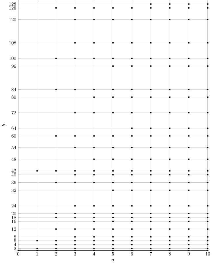
Answer (A special case of [BL92; BL93]).There are exactlypossibilities:
3.2. Finite arithmetic: the Burris-Lee theorem. Ordinary modular arithmetic remembers only a residue.
Exponentiation also needs a finite initial part in which small exponents remain distinct. The result is a finite arithmetic
with a tail followed by a cycle.
3.2.1. The Burris–Lee classification.
Definition 3.2.1 ().
For a natural number
and a positive integer ,
let be the
-element
quotient ,
where
Thus the numbers below
form the initial exceptional part, and the numbers from
onward repeat with period .
By [BL92, Proposition 3.6], every finite quotient of the positive integers has this tail–cycle form. The same paper
determines exactly when exponentiation descends to it.
Theorem 3.2.2 (Burris–Lee [BL92, Theorem 3.12]).Forand, the canonical operations
descend from toif and only if, for
every prime and every
positive integer ,
Burris and Lee work with the positive integers and the language
.2
3.2.2. Examples and the five cyclic models.
Example 3.2.3 (The rieg of truth values). The quotient
is the rieg of truth values
from Section 5.
Example 3.2.4 (Parity rieg). The quotient
is
which we call the parity rieg. Keeping
separate is essential: exponentiation does not descend to ,
since
is odd but
is even.
Example 3.2.5 (Overflow riegs). For ,
the quotient
is the overflow rieg with threshold ,
denoted by .
Its elements are ,
where every natural number at least
is sent to .
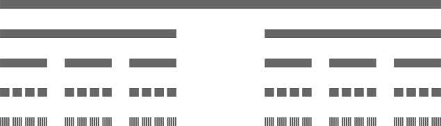
The theorem gives all finite quotient riegs at once. Figures 3 and 4 keep their distribution visible.
Figure 3. Finite quotient riegs of
for small
and
Figure 4. Finite quotient riegs of ,
arranged by
When , the
positive part has no tail: its successor operation is a single cycle. Following [AJ25], we call such positive algebras cyclic
models. There are surprisingly few of them.
Corollary 3.2.6 ([BL92, Corollary 3.14], attributed there to D. Higgs).The only finite quotient riegs ofwith
cyclic positive part are
Equivalently, if a rieg
has a least positive integer
such that
then
is one of .
This is precisely the puzzle in Section 3.1.3; no separate calculation is needed here.
Example 3.2.7.The number
satisfies both conditions in Theorem 3.2.2 with .
Hence
is a rieg. This is exactly the finite arithmetic used in the high-school calculation of Section 3.1.1.
Example 3.2.8. The number
fails the second Burris–Lee condition, since
but .
For every ,
however,
and ,
so
is a rieg. These riegs form the finite inverse system used below to construct the topological rieg of -adic
natural numbers (Definition 3.3.6).
3.2.3. Characteristics of riegs.
Recall that the characteristic of a ring
is the smallest positive integer
such that , if such an
exists; otherwise, the
characteristic is defined to be .
For quotient rigs and riegs, we need to record both the beginning of the cycle and its period. We order
by
Definition 3.2.9 (Characteristic). The characteristic of a rig or rieg
, denoted by
, is the
minimum pair
such that
if it exists. Otherwise, we put ,
where
is a formal maximum element.
Corollary 3.2.10 (Burris–Lee theorem in terms of rieg characteristics [BL92; BL93]).A pairis the
characteristic of a rieg if and only if
for every prime and every positive integer .
Remark 3.2.11 (Why this definition is natural).Let
be a rig or rieg. Factor the unique homomorphism from the initial object as
If this image is finite, then it is
and .
If the map
is injective, then .
The usual definition for rings cannot be used directly: if a positive integer
satisfies
in a rieg, then
is an additive inverse of ,
and the rieg is degenerate by Claim 2.3.1.
This viewpoint makes sense for any equational theory: for an algebra ,
the image of the canonical map from the initial algebra is a quotient of the initial algebra, and this quotient deserves
to be called the characteristic of
in general. For rings, the initial algebra is ,
the image is ,
and we recover the usual characteristic .
For riegs, the image is ,
and
is just a name for this quotient.
3.3. Profinite arithmetic: a total exponentiation.
In this subsection, we take the profinite completion of the initial rieg
and describe it explicitly. Its
underlying set turns out to be .
The main point is not that the exponentiation is total—this holds in every rieg by definition—but where it is total:
although no non-degenerate ring admits a rieg structure (Proposition 2.3.2), the completion contains the profinite ring
, and the
exponentiation
is still defined for all pairs.
3.3.1. Profinite natural numbers with total exponentiation.
For or
, let
denote the poset of
quotient -algebras
of . We put
if there is a quotient
map compatible with
the maps from .
Let
denote its subposet of finite quotients. Thus we use four notations, which form a square of subposets of
:
Going down-left in the square imposes the arithmetic condition of Theorem 3.2.2 (admitting a rieg structure); going down-right imposes
finiteness. The smallest poset ,
placed at the bottom, satisfies both conditions. Every finite quotient rig is of the form
. The finite quotient riegs are the ones
that satisfy Theorem 3.2.2, and
is the maximum element of each full quotient poset. For two finite quotients, the order is
Recall that the profinite completion of an algebraic structure is the limit of its finite quotient algebras
(Section A.2).
Definition 3.3.1.The rieg of profinite natural numbers
is the profinite completion of the initial rieg .
Thus
Lemma 3.3.2.The quotient rieg exists for every .
Moreover, the family
is cofinal in .
Proof.Suppose that is
prime and that , where
is maximal. Counting
the factors divisible by
gives
Moreover, if ,
then ,
so
divides .
Thus
is a rieg by Theorem 3.2.2.
Now let be a finite
quotient rieg and take .
Then
and , so
This proves cofinality. □
Proposition 3.3.3.The profinite rieg is the limit of the following diagram.
Proof.By Lemma 3.3.2, the order-preserving functor
is final. Therefore, it gives the same limit. □
Theorem 3.3.4 (The underlying set of ).The underlying set of is
where denotes the usual set of profinite
integers. The canonical projection restricts to the canonical maps
and
Proof.By Proposition 3.3.3 and lemma A.2.1, an element of
is a
compatible sequence
Suppose that one coordinate is an exceptional element
.
Compatibility then gives
Hence the sequence comes from the natural number
. Otherwise, every coordinate
belongs to the modular part ,
so the sequence is an element of
Conversely, every element of
and every element of
gives a compatible sequence of the indicated form. □
Figure 5. as
limits of
Corollary 3.3.5 (The unique continuous extension of exponentiation).The exponentiation ofextends
to a continuous operation
defined for all pairs of elements, and such a continuous extension is unique.
Proof.The limit defining
is taken in the category of topological riegs. Hence its operations, including exponentiation, are defined
coordinatewise and are continuous by Lemma A.2.1.
For the uniqueness, it suffices to show that the image of
is dense in :
then
has dense image in ,
and two continuous maps into the Hausdorff space
that agree on a dense subset must coincide. By Proposition 3.3.3, every non-empty basic open subset of
is the preimage of a non-empty subset
under the projection
for some .
Since the composite
is surjective, this preimage contains an element of .
□
This is different from the usual -adic
exponentiation, which is not defined on all pairs in .
In fact, a non-degenerate ring cannot be a rieg by Proposition 2.3.2. The summand
in Theorem 3.3.4
is what makes
different from a ring.
By using a smaller diagram of finite quotient riegs, we obtain variants of
. The
following one appeared in Phenomenon 2 (Section 3.1.2).
Definition 3.3.6 (The topological rieg of -adic natural numbers). The topological rieg of -adic
natural numbers
is the limit of the following diagram in the category of topological riegs:
By the same argument as in Theorem 3.3.4, the underlying set of
is given
by
where denotes
the set of -adic
integers.
Remark 3.3.7 (No -adic analogue).This construction does not work for the powers of a single odd prime, say :
since
but ,
the second condition in Theorem 3.2.2 fails. Hence the rig
admits no rieg structure for any .
In this sense, there is no topological rieg of “-adic
natural numbers”
obtained in this way.
3.3.2. Contractive exponential dynamics.
Definition 3.3.8 (Carmichael function [Car10]). For a positive integer
, the Carmichael
function is the least
positive integer
such that
for every .
Equivalently,
is the exponent of the group .
Remark 3.3.9 (The jump function). With respect to the divisibility order, the Carmichael function has a right adjoint
, whose
notation
we borrow from [CP09, Theorem 5.2(b)]. Thus
Therefore,
records the possible next periods
for which exponentiation raises the precision.
Lemma 3.3.10 (A metric for an inverse sequence).Let
be an inverse limit of non-empty finite sets and surjective maps, wherehas one element. Writefor the projections.
For distinct ,
let
and put
Thenis a complete ultrametric space.
Suppose that a map satisfies
for every .
Then is a contraction with Lipschitz constant .
Proof.The ultrametric inequality follows because two elements that agree with a third element through level
also agree with each other through level .
A Cauchy sequence stabilizes at every finite level. These stable coordinates form an element of ,
so the metric is complete.
If and
agree through
level ,
then and
agree through
level .
Hence
□
We now use another inverse sequence for the same topological rieg:
All the displayed objects are quotient riegs by Theorem 3.2.2. Adding the last four quotients does not change the limit in
Definition 3.3.6. The periods in this sequence are
The standard formula for the Carmichael function [Car10] gives
and
The modular parts of this inverse sequence have limit
We equip this limit with the metric in Lemma 3.3.10. Since
is a
topological rieg, its total exponentiation defines a map
This map preserves the modular part: at each finite quotient, a modular exponent can be represented by an integer
above the
tail, and
is again above the tail. If two elements of the modular part agree modulo a period
, then their images agree
modulo the next period :
indeed, and
is invertible
modulo .
Therefore,
raises the agreement by one level. By Lemma 3.3.10, the restriction
is a contraction with Lipschitz constant .
Lemma 3.3.11 (Stabilization of the last two digits).For every element of the modular part ,
we have .
Proof.The first four transitions of the above sequence give
and then
□
Proposition 3.3.12 (The unique fixed point of ).The function on has a unique fixed point ,
which belongs to ,
and every iteration sequence starting from converges to .
Furthermore, for each ,
the reduction of is the unique solution of in (cf. Figure 1).
Proof.There is no fixed point in the natural-number part, since
for every .
On the modular part, the map
is a contraction on a non-empty complete metric space. The Banach fixed-point theorem gives a unique fixed point
,
and every iteration sequence in the modular part converges to .
It remains to prove the statement at each finite level. If
satisfies
, then
by Lemma 3.3.11. Suppose that the solution is unique modulo
, and let
and
be solutions
modulo . Their
reductions modulo
coincide. Since ,
we obtain
Hence the solution is unique at every level. The reduction of
gives its existence. □
We close this subsection by determining the solutions of another exponential equation,
, in the
same topological rieg.
Proposition 3.3.13 (The solutions of ).In , the equationhas exactlysolutions: the
element of the
summand ,
and the ten elements
of ,
where denotes the group of fourth roots of unity in .
Proof.In the summand ,
we have ,
,
and
for ,
so
is the only solution there.
Let belong to
the modular part ,
let , and choose
an integer
with . Since
is a rieg (Example 3.2.8),
the reduction of
to is
.
Therefore,
Below,
denotes the -adic
valuation and
ranges over .
First, suppose
and put .
Taking
in , we
have ,
and with
and
, so
and
contradicting .
Hence each of the two coordinates of
is either
or a unit.
Next, suppose that the -coordinate
of
is a unit. Then
modulo
reads ,
i.e., the order of
in
divides .
If ,
it is a torsion element of ;
assume
and put .
Once ,
we have .
For ,
the order of
is a power of
dividing ,
hence divides .
For ,
the order divides ;
its -part
divides ,
hence divides ,
while its prime-to-
part divides .
In both cases the orders are bounded independently of ,
so
is a torsion element of .
The torsion subgroup of
is ,
and that of
is .
Finally, we determine which of the remaining
combinations satisfy ;
note that the same representative
serves both coordinates. If the -coordinate
is ,
then ,
so
is odd, and the order of the -coordinate
must be odd: the -coordinate
is
or .
If the -coordinate
is ,
then ,
so every order in
divides :
the -coordinate
can be any element of .
If the -coordinate
is ,
then ,
so :
the order
divides
but
does not, and the -coordinate
lies in .
This yields the
listed elements. Conversely, each listed element satisfies :
a coordinate
gives ,
hence ,
and the case analysis above shows precisely that the order of each torsion coordinate divides .
□
Remark 3.3.14 (The levelwise counts diverge). Contrast Proposition 3.3.13 with
Proposition 3.3.12, where every level has a unique solution. The numbers of solutions of
in
for
are
and they are unbounded, even though the limit has only
points: for a unit
with ,
one has ,
so
solves the -adic
part of the equation modulo
precisely when .
Pairing such
with the -coordinate
produces, for ,
at least
solutions at level ,
almost all of which die at a later level. Note also that
is a solution in the summand
but not in the summand :
modulo ,
the class
is represented by ,
and .
This illustrates the splitting
of Definition 3.3.6.
4. Example 2: Riegs in category theory and combinatorics
In this section, we consider the rieg structures obtained through decategorification. Since many of these are defined via
universality, the verification of the rieg structure follows from abstract nonsense. However, when one tries to write them
down explicitly, it looks non-trivial that all fourteen axioms of a rieg are satisfied.
For example, from abstract nonsense, it follows immediately that the set of all isomorphism classes of finite directed graphs
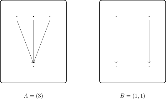
admits a natural rieg structure. But can you imagine what the exponentiation looks like? For instance, consider a single
edge ,
and then consider taking the exponential of that edge with itself, denoted
.
The resulting graph is depicted in Figure 6: its four vertices are the four functions from the vertex set
of
to itself (the two
constant functions ,
the identity , and
the transposition ),
and it has exactly four edges, one of which is a loop. Notice that the vertex
is
isolated.
Figure 6. The exponential graph
Regarding the decategorified semiring structure, numerous studies have been conducted under the name Burnside rig.
However, to the author’s knowledge, research on its exponential structure has been very limited. Despite the
exponential structure satisfying numerous equations in the definition of rieg, these have been left unused. See
[Sch00b]
4.1. Burnside rieg of CCC with finite coproducts (and a topos).
4.1.1. The Burnside rieg functor .
Definition 4.1.1.The (-)category
is
defined as follows:
Its objects are small categories that are cartesian closed and have finite coproducts.
Its morphisms are functors between these categories that preserve finite products, finite coproducts, and
exponentials, where we consider functors up to natural isomorphism3 .
Proposition 4.1.2.For a cartesian closed categorywith finite coproducts, the set of isomorphism classes offorms a rieg with the categorical initial object, the binary coproducts, the terminal object, the binary products, and
the exponentials.
Proof.All of the fourteen axioms are implied by the universalities. □
Remark 4.1.3 (Symmetric monoidal closed categories).This construction does not work for a symmetric monoidal
closed category with finite coproducts, since we use the fact that the product
is a categorical product to prove some axioms including .
We borrow the following notation from [Men17] (and from [Sch90]).
Definition 4.1.4.The Burnside rieg functor
sends an object
of the category
to the rieg induced by
(Proposition 4.1.2), and a functor in
to the induced rieg homomorphisms.
Proposition 4.1.5 (Topos to rieg functor).For a locally cartesian closed small categorywith finite coproduct (in
particular, an elementary topos ),
the correspondence
defines a contravariant functor
Example 4.1.6 (Finite sets to natural numbers). The Burnside rieg of finite sets is isomorphic to the rieg of natural
numbers
Example 4.1.7 (Infinite sets to cardinal arithmetic). Let
be an infinite cardinal and
be the (essentially small) category of sets with cardinality less than .
The category
is a topos if and only if it is cartesian closed if and only if
is a strong limit cardinal. Therefore, if
is a strong limit cardinal, then we obtain the induced rieg ,
which is the (small) rieg of cardinal arithmetic.
Obviously, the structure of this rieg is interconnected with set theory, especially continuum hypothesis. With the
generalized continuum hypothesis,
is a countable rieg with .
However, without the GCH, there are many other possibilities of this rieg structure.
Example 4.1.8 (Finite presheaf topos).For any small category
,
has all finite limits and colimits.
Therefore, if is cartesian closed,
we obtain a rieg . For example,
if is a finite category or a
(possibly infinite) group, then
is known to be cartesian closed (and a topos).
The category of finite functions
forms a rieg of multisets of natural numbers (or Dirichlet polynomials [SM23]).
More generally, for any finite category ,
its finite (co)presheaf category
forms a rieg. Examples include the category of finite graphs
and the category of rooted forests .
For any (possibly infinite) group ,
the category of its finite actions
forms the Burnside rig of the group .
Examples include the category of sets with involution
and the category of finite loops .
On the other hand, the category of finite discrete dynamical systems
is not
cartesian closed.
Question 4.1.9.When is a finite presheaf categorycartesian closed? The author is also interested in the closely related question: when is a finite presheaf category a
topos?
Example 4.1.10.
Every Heyting algebra
is a cartesian closed poset with finite coproducts, and thus a rieg.
4.1.2. Enumerations. In many cases, to utilize the Burnside rieg
to enumerate something, we
consider a enumeration function ,
which is typically a rig homomorphism. There are several ways to choose such enumeration function.
Example 4.1.11 (Global sections for a connected topos).For example, for a locally finite topos
we have the global section functor ,
which preserves products, but not necessarily coproducts. If the topos
is connected (i.e., if
preserves finite coproduct), then the functor
induces the rig homomorphism
that counts the number of global sections.
Example 4.1.12 (Connected components for a stably locally connected topos).If a topos
admits an adjoint triple
such that
preserves finite products (see stable local connectedness in [Joh11]), then the functor
induces a rig homomorphism .
Example 4.1.13 (Enumeration with a torsion-free atom.).Let
be a small topos. Due to Proposition 4.1.5, every object
induces a rieg homomorphism .
Therefore, if ,
then we obtain a rieg homomorphism .
According to the terminology in [KM91], we call such an object
a torsion-free atom4 .
4.2. Riegs of functions :
List of numbers and Liouville’s divisor theorem.
4.2.1. The Burnside rieg of functions .
Our first example is the Burnside rieg of the topos ,
which is called the topos of (finite) fucntions or the (finite) Sierpinski topos. An object of the topos is a function
.
Since a function can be
regarded as a family of sets , the
isomorphism classes of the topos
are in bijective correspondence with the finite multiset of natural numbers. Let
denote the set of all multisets of natural numbers. Each multiset will be denoted as a list of natural numbers
, and rearranged
lists are identified .
The addition is given by a concatenation of lists, and the product is given by the list of all ccomponent-wise
products.
[SM23] explains that this rig structure is isomorphic to the rig of (formal) Dirichlet polynomials
However, exponentials are different:
There is a unique extension of this exponential to all exponentials. For example,
Remark 4.2.1 ( and Artin gluing).
4.2.2. Liouville’s theorem.
The equation
is well-known. As studied in [BS13], there are so many similar equations including
,
,
and
.
So the question is: for a given finite list of natural numbers
, does the
equation
(1)
holds?
Writing for the number of
divisors of a positive integer ,
Liouville’s theorem states that
For example, in the case of ,
we obtain the equation
The proof of this theorem is not difficult, and is just a highschool level problem. Given the equation
, it suffices to prove that the problem
can be reduced to the case of
for some prime number .
In other words, the only non-trivial part is to prove that if two sequence
and
satisfies the equation, so does
their “product sequence” .
Here is a categorified (or Burnside) point of view. Consider the Burnside rieg
of the
topos of functions between finite sets. We obtain the equivalence
Figure 7. The representing object of sum-of-cubes and square-of-sum in
4.3. Rieg of finite groups.
Counting problems. We will give a rieg-theoretic method to answer the following undergraduate-level counting
problems.
Question 4.3.1.For a finite group ,
let denote the number of subgroups whose index (= the number of cosets) is .
Write using and .
Question 4.3.2.Count the number of group homomorphisms from to itself. (Hint: is the dihedral group of order ,
and .)
Notice that all operations of the cartesian
closed category of finite groupoids are well-defined
up to equivalence. Therefore, (as a -categorical
analogy of Proposition 4.1.2), the equivalence classes of finite groupoids, which are the formal sums of finite groups, form a
rieg! The aim of this section is to concretely describe the rieg structure.
Definition 4.3.3.We definite the rig of finite groups
as follows:
The underlying additive commutative monoid is the free commutative monoid of the set of isomorphism classes of
finite groups, which is given by the finite formal sum.
The multiplication is given by the unique extension of
Hereafter, the isomorphism class of a group
will be simply referred to as .
Notation 4.3.4.The (isomorphism class of) the cyclic group
is denoted by .
Example 4.3.5.Some examples of calculations include:
Definition 4.3.6 (Conjgacy classes of homomorphism).Let
and
be finite
groups.
Two homomorphisms
are conjugate if there exists
such that
holds.
The automorphism group (or the stabilizer) of a homomorphism
is the subgroup of ,
defined by .
Theorem 4.3.7.The rig of finite groups admits the following rieg structure:
For two finite groups and , its
exponential is defined by
In general, the exponential is defined by
for any two families of finite groups and .
Proof.This is the rieg of equivalent classes of finite groupoids, explained at the beginning of this section. □
Example 4.3.8. Let’s try to calculate .
In order to utilize the exponential rules, we first calculate smaller parts:
Then we obtain
Some properties of finite groups, like being abelian, are characterized in terms of this rieg structure.
Proposition 4.3.9.For a finite group ,
if is abelian, then we have
conversely, if is a sum of for any ,
then is abelian.
Proof.The former statement is immediate from the definition. If
is a sum of
for any ,
then
is a sum of .
Especially, we have
and
is abelian. □
Now we can answer the first problem, Question 4.3.1!
Remark 4.3.10.For a limit cardinal ,
one can consider a rieg of larger groups, in which we can similarly consider representations of product groups, like
.
4.3.1. Groupoid cardinality. In order to utilize riegs for counting something, the basic rieg
theoretic method is to consider a rig homomorphism from a given rieg to the rig of numbers, like
.
For the rieg of finite groups ,
the notion of groupoid cardinality, introduced in [BD01], is useful. We can utilize it to obtain rational numbers from elements of
.
Definition 4.3.11.For ,
its groupoid cardinality
is defined by
Proposition 4.3.12.The groupoid cardinality functionis a rig homomorphism.
Furthermore, for finite groups and , we
have
Proof.For sums and products, the proof is easy. Regarding exponentials, one can use the orbit-stabilizer theorem for
the conjugate action of
on .
□
Exercise 4.3.13.Check that Proposition 4.3.12 is compatible with Proposition 4.3.9.
Let us finish this introductory note by giving the answer to Question 4.3.2!
Answer (to Question 4.3.2).In Example 4.3.8, we obtained. By
taking the groupoid cardinality, we obtain
This proves that .
5. Example 3: Riegs in logic
In this subsection, we investigate the riegs that consist of “propositions.” The motivating examples are the rieg of truth
values and the rieg of subsets:
Example 5.0.1 (Rieg of truth values).The set of truth values
has a natural rieg structure, as .
This is isomorphic to the overflow rieg with threshold
and .
Example 5.0.2 (Powerset). For any set ,
its powerset
has a rieg structure with ,
where
is defined to be .
More generally, every Heyting algebra5
is a rieg.
When ,
its powerset rieg is the degenerate rieg. When
is a singleton, its power rieg is the rieg of truth values.
The above riegs have special properties:
The underlying rig is a lattice
They are Heyting algebras.
For each property, we have a class of riegs. We will study them one by one.
5.1. Riegs in which .
Proposition 5.1.1.For a rieg ,
the followings are equivalent:
(1)
(2)
or
(3)
There is a rieg homomorphism from the rieg of truth values
(4)
The addition is idempotent. (i.e., for any ,)
(5)
Both addition and multiplication are idempotent. (i.e, for any ,)
Proof.The equivalence between 1, 2 and 3 follows from the definition of characteristics. By multiplying
, we have
14. To prove
5 from ,
we can use
The remaining implications are trivial.
□
Example 5.1.2 (Max-plus is not a rieg).The max-plus algebra
admits no rieg structures. If it admits a rieg structure, since ,
the multiplication ,
(which is the addition in the usual sense) should also be idempotent. However, ,
contradiction.
Definition 5.1.3. A rieg
is said to be idempotent, if it satisfies the conditions of Proposition 5.1.1.
Remark 5.1.4.(Multiplicatively idempotent riegs) Even if a rieg
is multiplicatively idempotent, it might not be additively idempotent. For example, the parity rieg Example 3.2.4
is multiplicatively idempotent but not additively idempotent.
However, there is a strong restriction on the characteristics. For a multiplicatively idempotent rieg
, its characteristics
should be
less than
since .
Therefore, there are only finitely many possible characteristics, namely
And all of them are possible, since
are multiplicatively idempotent.
5.2. Riegs that are lattices. Next, we will study when (the underlying rig of) a rieg is a lattice. The necessary condition
is being idempotent (Definition 5.1.3). However, this is not sufficient:
Example 5.2.1 (Idempotent rieg that is not a lattice). In Example B.1.9, we observed that
with
exponential
is a rieg.
Dividing
into
groups
we obtain a -element rieg
as a quotient rieg. Indeed, the group
to which belongs is determined
by the pair of data (whether
or ; whether
is constant or increasing),
and this pair for and
for is determined
by the pairs for and
(for the multiplication,
note that consists of the
single element ). For the
exponential, observe that
is equal to if
, and belongs to the
same group as if
; in both cases, the
group of depends
only on the groups of
and .
The underlying rig of this quotient is the rig presented by a single generator
and two
equations and
. (The additive idempotency
follows from via
; hence the presented rig
consists of the four elements ,
and , corresponding
to , and
, respectively.) This rieg
satisfies , but the underlying
rig is not a lattice since .
Proposition 5.2.2 (Rieg and Lattice).For a rieg ,
the following conditions are equivalent:
(1)
The underlying rig is a (bounded) lattice.
(2)
For any ,.
Proof.The implication
follows from the fact that
is the maximum element in a lattice.
We prove 1 from 2. Substituting
with , we
obtain ,
i.e., this rieg is idempotent (Definition 5.1.3). Now it is enough to prove the absorption laws
It is proven as .
□
5.3. Heyting algebras are riegs. A Heyting algebra is not just related but is a rieg satisfying additional
equations.
Proposition 5.3.1.Every Heyting algebrais a rieg.
Proof.We can directly prove this. Alternatively, this is also an immediate corollary of Proposition 4.1.2, since a
Heyting algebra is a bicartesian closed category whose underlying category is a poset. □
Example 5.3.2 (A rieg that is a lattice but not a Heyting algebra).Let
be the power set of a non-empty set ,
equipped with a rig structure given by
and .
We consider a rieg structure on
that is different from Example 5.0.2.
First, fix an arbitrary element
and define the exponential as
This rieg structure is given by the composition of two rig homomorphisms. The first one is a rig homomorphism to the rig of
truth value
defined as
The other is the unique rig homomorphism
which sends to the
constant funciton
and to the
identity function .
Remark 5.3.3 (Riegs from ultrafilters). Rig homomorphisms
correspond exactly to ultrafilters on .
For each ultrafilter
on ,
the same construction equips the rig
with a rieg structure: the exponentiation is given by
if ,
and
otherwise. The example above is the special case where
is the principal ultrafilter generated by .
If has
at least two elements, this rieg is not a Heyting algebra, because
Proposition 5.3.4.A rieg is a Heyting algebra, if and only if it satisfies the following additional equations:
Corollary 5.3.5.The category of Heyting algebras is a reflective full subcategory of the category of riegs .
The construction of the left adjoint is the usual one: quotient by new equations. For example, the associated Heyting algebra of
is the Heyting algebra of truth values
6
The relation between Heyting algebras and riegs is not an addition of structures, but an addition of properties. In this
respect, it is closer to the relationship between abelian groups and groups rather than to the relationship between rings and
groups.
Appendix A. Preliminaries on equational theory and profinite topology
In this section, let
be a (finite arity single-sorted) algebraic theory. We are especially interested in the case
. The category
of -algebras is
denoted by .
A.1. Categorical properties of riegs (and general-algebras).
Remark A.1.1 (Categorical properties of riegs).Several category-theoretic properties of
immediately follow from the mere existence of an equational definition by the theory of categorical universal algebra. Some
of them are noted below.
The category of riegs
has all small limits and colimits.
Furthermore, the forgetful functor
(preserves and) creates all limits.
The forgetful functor
has a left adjoint
Every rieg homomorphism
is uniquely (up to the canonical isomorphism) decomposed into the composition of a surjective homomorphism
followed by an injective homomorphism .
This means we can construct arbitrary small limits using limits in
. For a given family of riegs
, its categorical product is
given by the product set
with the index-wise operations.
An element of the free rieg
looks like
A.2. Topological -algebras
and their profinite completion.
A topological -algebra
is a model of in the
category , that is, a
-algebra equipped with a topology such
that all operations of are continuous.
Morphisms of topological -algebras are
continuous -algebra homomorphisms.
The category of topological -algebras
is denoted by .
It is straightforward to verify the next lemma.
Lemma A.2.1 (Limits in the topological -algebras).admits all small limits, which are preserved by the two forgetful functors and .
In otherwords, a small limit in
is just the limit at the underlying set level equipped with the canonical
-algebra
structure and the initial topology.
For a given -algebra
, a quotient
-algebra is a
surjective -algebra
homomorphism ,
up to the canonical isomorphisms. The quotients form a complete lattice
. We put
if there exists a homomorphism
that commutes with the
quotient maps from . Let
denote the subposet of
finite quotient -algebras.
Definition A.2.2 (Profinite completion of a -algebra).For a -algebra
, its profinite completion
is the limit of all
finite quotients of .
In other words,
is the limit of the following diagram:
Remark A.2.3 (As a codensity monad).It is much more natural to define the profinite completion as an endofunctor
on the category
although we will not need it in the present paper. The category of finite (and discrete) -algebras
is a full subcategory of the category ,
and the codensity monad of the embedding
is the profinite completion.
Appendix B. Other (counter)examples
B.1. Basic examples.
Example B.1.1 (Non-negative real numbers).The set of non-negative real numbers
has the
natural rieg structure, defining
The rieg of natural numbers is a subrieg of this rieg. However, the subset of all non-negative rational numbers is
not subrieg, since it is not closed under exponentials.
Proposition B.1.2 (J. Koizumi, personal communication).Letpreserve
the exponentiation, i.e. satisfy
Thenis either the constant functionor the identity function.
Proof.Putting ,
the value
satisfies ,
hence
and .
Applying to
gives
Assume
is not constantly ,
and fix
with ;
then ,
i.e.
is multiplicative. Put
for .
Multiplicativity gives ,
while the original equation with
gives
for all
and .
Fixing
with ,
we obtain ,
so additivity of
makes
additive: .
An additive function with positive values is strictly increasing, and
forces
for every positive rational ;
being increasing and agreeing with the identity on a dense subset, .
Conversely, both functions do satisfy the equation. □
Remark B.1.3.The hypothesis has to be ,
that is,
is an endomorphism of the binary operation .
Under the weaker reading
the statement is false, since
satisfies
for every .
Note also that
is not a rieg, having no ;
it is a model of the eleven high school identities, so the correct reading of Proposition B.1.2 is a rigidity statement
about -endomorphisms.
Remark B.1.4 (The rig is not a rieg). It is natural to ask whether this rieg structure can be extended to the rig .
The answer is no. The rig
cannot have a rieg structure. Suppose that there is an extension to a rieg structure. First, since ,
we have .
And, since ,
we have ,
contradiction.
B.1.1. Numbers with Infinites.
Example B.1.5 (Complemented natural numbers).
has a canonical rieg structure, which is obtained as the limit of the overflow riegs
In this sense, this rieg is the overflow rieg with threshold .
Notice that this construction is similar to the construction of -adic
integers.
B.1.2. Rig with many rieg structures.
Example B.1.6 (Rieg of dual numbers constructed by Yuhi Kamio). Recall that a dual number is a number plus an
“infinitesimal number”
The ring of infinitesimal numbers is denoted by
and algebraically defined as
There is a similar rieg, which we call the dual number rieg.
Definition B.1.7 (Dual numbers, concrete definition). The dual number rieg
has
as the underlying
set and its element
is denoted by .
Three operations are defined as follows:
(1)
(2)
(3)
The exponential depends only on the natural-number part
of the exponent:
This definition has a more conceptual paraphrase, with which we can easily prove that it’s actually a rieg. First notice
that the projection
is a rig homomorphism to the initial rig .
Thus we have the composite rig homomorphism
and this gives the exponential structure of the dual number rieg.
More generally, we have the following proposition.
Proposition B.1.8 (Rieg structure by a natural number evaluation).For a commutative rigand a
rig homomorphism (or say, “natural number evaluation”)
admits an induced rieg structure
In other words, the exponential is given by
For example, we can replace the additive group
in the definition of the dual number rieg with an arbitrary commutative monoid.
Example B.1.9. In Proposition B.1.8, letting
be the evaluation function
we have a rieg structure on
with
Example B.1.10 (Rieg of polynomials). Is it possible to have more than one rieg structure on
a single rig? The answer is (not at all surprisingly) yes. A typical example is the rig of polynomials
. Since
is the free rig with
a generator , rieg
structures on
bijectively correspond to the elements of
B.2. Riegs of three elements. The degenerate rieg
is the unique -element rieg. The
rieg of truth values is the unique
-element rieg. This subsection
aims to provide all -element
riegs.
Proposition B.2.1 (-element riegs).There are isomorphism classes of -element
riegs.
Let be a
-element rieg. There are three
possible characteristics .
Case 1: . If
, then
is the parity rieg (Example 3.2.4) or the overflow rieg with the threshold
(Example 3.2.5).
Case 2: . So we need to
classify all -element riegs
with characteristics .
Let . We distinguish
cases based on the value of .
- Case 2.1: and . If
, then the rieg
satisfies the equation
, which means that
the underlying rig of
is the lattice
(Proposition 5.2.2). This rig
is isomorphic to the rig
Therefore, the rieg structures
on the rig
are in bijective correspondence with the monoid homomorphisms
, which correspond to the
exponentiation function ,
that satisfy
,
which always holds,
,
and
.
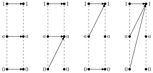
In other words, the rieg structures on the rig are in bijective
correspondence with the idempotent -semilattice
homomorphisms with
. One can show that
there are exactly rieg
structures on the rig ,
which are visualized in Figure 8.
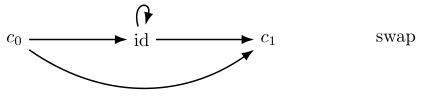
Figure 8. The four possible exponentiations
- Case 2.2: and . The only
remaining case is ,
since is impossible
(Claim 2.3.1). Since
is idempotent (Definition 5.1.3), the underlying rig structure is determined:
Therefore, the rieg structures on
are in bijective correspondence with monoid homomorphisms
with
,
which always holds
,
and
.
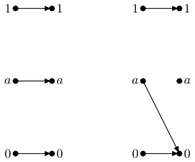
There are two such morphisms visualized in Figure 9.
Figure 9. The two possible exponentiations
References
[AJ25]
Tumadhir Alsulami and Marcel Jackson. “Cyclic arithmetic and combinatorial operations”. The
American Mathematical Monthly 132.4 (2025), pp. 316–332. doi: 10.1080/00029890.2024.2439803.
[BD01]
John C. Baez and James Dolan. “From finite sets to Feynman diagrams”. Mathematics
unlimited—2001 and beyond (2001), pp. 29–50.
[BS13]
Edward Barbeau and Samer Seraj. “Sum of cubes is square of sum”. Notes on Number Theory and
Discrete Mathematics 19.1 (2013), pp. 1–13.
[BHT09]
Jan A. Bergstra, Yoram Hirshfeld, and John V. Tucker. “Meadows and the equational
specification of division”. Theoretical Computer Science 410.12–13 (2009), pp. 1261–1271. doi:
10.1016/j.tcs.2008.12.015.
[Bir42]
Garrett Birkhoff. “Generalized arithmetic”. Duke Math. J. 9.1 (1942), pp. 283–302.
[BL92]
Stanley Burris and Simon Lee. “Small models of the high school identities”. International Journal of
Algebra and Computation 2.02 (1992), pp. 139–178. doi: 10.1142/S0218196792000104.
[BL93]
Stanley Burris and Simon Lee. “Tarski’s high school identities”. The American Mathematical Monthly
100.3 (1993), pp. 231–236.
[BY05]
Stanley N. Burris and Karen A. Yeats. “The saga of the High School Identities”. Algebra Universalis
52.2–3 (2005), pp. 325–342. doi: 10.1007/s00012-004-1900-2.
Robert D. Carmichael. “Note on a new number theory function”. Bulletin of the American
Mathematical Society 16.5 (1910), pp. 232–238. doi: 10.1090/S0002-9904-1910-01892-9.
[FDB06]
Marcelo Fiore, Roberto Di Cosmo, and Vincent Balat. “Remarks on isomorphisms in typed lambda
calculi with empty and sum types”. Annals of Pure and Applied Logic 141.1-2 (2006), pp. 35–50.
[Hit20]
Markus Hittmeir. “A reduction of integer factorization to modular tetration”. International Journal
of Foundations of Computer Science 31.4 (2020), pp. 461–481. doi: 10.1142/S0129054120500197.
Peter T. Johnstone. “Remarks on punctual local connectedness”. Theory Appl. Categ 25.3 (2011),
pp. 51–63.
[KM91]
Anders Kock and Ieke Moerdijk. “Presentations of étendues”. Cahiers de topologie et géométrie
différentielle catégoriques 32.2 (1991), pp. 145–164.
[Men17]
Matías Menni. “Every rig with a one-variable fixed point presentation is the burnside rig of a
prextensive category”. Applied Categorical Structures 25 (2017), pp. 663–707.
[OEIa]
OEIS Foundation Inc. Sequence A133613: Decimal digits such that for all ,
the number satisfies the congruence .
The On-Line Encyclopedia of Integer Sequences. url: https://oeis.org/A133613.
[OEIb]
OEIS Foundation Inc. Sequence A183613: modulo .
The On-Line Encyclopedia of Integer Sequences. url: https://oeis.org/A183613.
[Sch90]
Stephen H. Schanuel. “Negative sets have Euler characteristic and dimension”. Category Theory:
Proceedings of the International Conference held in Como, Italy, July 22–28, 1990. Springer. 1990,
pp. 379–385.
[Sch00a]
Stephen H. Schanuel. “Objective number theory and the retract chain condition”. Journal of Pure
and Applied Algebra 154.1-3 (2000), pp. 295–298.
[Sch00b]
Stephen H. Schanuel. Transcendence in objective number theory. 2000.
[SM23]
David I. Spivak and David Jaz Myers. “Dirichlet polynomials form a topos”. The Graduate Journal
of Mathematics 8.2 (2023), pp. 73–87.
[Wil00]
Alex J. Wilkie. “On exponentiation—a solution to Tarski’s high school algebra problem”. Connections
between Model Theory and Algebraic and Analytic Geometry. Ed. by Angus Macintyre. Vol. 6. Quaderni
di Matematica. Circulated as an Oxford University preprint in the early 1980s. Rome: Aracne, 2000,
pp. 107–129.
Theorem Let \(R\) be a compact Hausdorff topological rieg. If its additive commutative monoid is cancellative, then \(R\) has one element. Connectedness is not required. Lemma Every compact Hausdorff commutative cancellative topological monoid \((S,+,0)\) is a group. Proof. First …
Question Does a nontrivial connected compact Hausdorff topological rieg exist? All three binary operations—addition, multiplication, and exponentiation—are required to be continuous. Current result Compact rieg no-go proves that every compact Hausdorff topological rieg with …
Enable SUMIRE in your conversation. If the request is not filled in, paste the copied request. If the app does not open, install it or use its website.