SUMIRE Sign in

The starting point is Games as recursive coalgebras: A categorical view on the Nim-sum, available in Main. The paper develops impartial games as recursive finite-powerset coalgebras, game values as recursive evaluations, and Bouton monoids as universal factorizations of game values. Conway addition is symmetric monoidal closed.

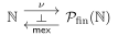
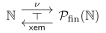
The next question is how much more explicit this framework can become. The internal hom has a proposed concrete cofree-subgame construction and proof in note 29; its relationship to playing strategies remains separate. Differential structures asks for a common explanation of the Leibniz-type move formula and the Rota–Baxter-type law, with an explanation of Nim-sum as the target.

Two extensions have different starting points. Partisan games already recover short game forms, but values and strategies need additional structure. A double category of games still requires a precise strategy class and compatible squares; counterexamples for arbitrary relations do not settle that question.

A settled boundary is that Game itself is not a topos, by Remark B.27 of the paper. Questions about a topos completion are therefore distinct from that answered question.

To contribute, choose one of these linked questions and work against its stated remaining claim. For the internal hom, compute a small explicit example or clarify its game-theoretic meaning. For the double category, specify legal strategies and test compatibility with coalgebra maps before claiming a general construction or obstruction.

Games as recursive coalgebras
A categorical view on the Nim-sum

Ryuya Hora Address: ZEN University, Japan Email address: ryuya_hora@zen.ac.jp
Date: August 24, 2026
Abstract.

In 1901, Bouton proved that a winning strategy for the game of Nim is given by the bitwise XOR, called the nim-sum. But why does such a weird binary operation work? Led by this question, this paper introduces a categorical reinterpretation of combinatorial games and the nim-sum. The main categorical gadget used here is recursive coalgebras, which allow us to redefine games as “graphs on which we can conduct recursive calculations” in a concise and precise way.

For game-theorists, we provide a systematic framework to decompose an impartial game into simpler games and synthesize the quantities on them, which generalizes the nim-sum rule for the Conway addition. To read the first half of this paper, the categorical preliminaries are limited to the definitions of categories and functors.

For category theorists, this paper offers a nicely behaved category of games 𝐆𝐚𝐦𝐞\mathbf{Game}, which is a locally finitely presentable symmetric monoidal closed category comonadic over 𝐒𝐞𝐭\mathbf{Set} admitting a subobject classifier!

As this paper has several ways to be developed, we list seven open questions in the final section.

Key words and phrases:
Impartial games, nim-sum, Conway addition, recursive coalgebra, hylomorphism, monoidal category, monoid, locally presentable category, subobject classifier.
2020 Mathematics Subject Classification
91A46, 18C50, 03B70

Throughout this paper, ℕ\mathbb{N} denotes the set of all non-negative integers ℕ={0,1,2,…}\mathbb{N}=\{0,1,2,\dots\}.

1. Introduction

1.1. Why does the nim-sum appear?

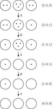
In 1901, Bouton discovered the remarkable (and now very famous) winning strategy of the game nim in [Bou01]. In nn-heap nim, there are nn heaps of stones, with a1,…,ana_{1},\dots,a_{n} stones in each heap. Two players take turns removing stones, but on each turn, they must remove stones from one heap (and “removing 00 stones” is not allowed.) The player who can no longer make a move loses11 1 Usually, the rule is stated as “the player who takes the last stone wins,” but it does not make sense in the particular situation where a1=a2=⋯=an=0a_{1}=a_{2}=\cdots=a_{n}=0 from the start.. For example, Figure 1 is a typical play from the state (a1,a2,a3)=(2,3,3)(a_{1},a_{2},a_{3})=(2,3,3), where AA wins.

(2,3,2); (2,3,1); A; (1,3,1); B; (1,0,1); A; (1,0,0); B; (0,0,0); A
Figure 1. A play of 33-heap Nim, where AA wins.

Bouton’s winning strategy is based on a nicely designed group structure on ℕ\mathbb{N} called nim-sum. (We will define the nim-sum again in a more formal way in Definition 2.16.)

Definition 1.1.

The nim-sum of two natural numbers is the bit-wise excluded disjunction.

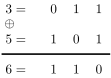
For example, the nim-sum of 33 and 55 is 66 (Figure 2).

3=; 0; 1; 1; 5=; 1; 0; 1; 6=; 1; 1; 0; ⊕
Figure 2. Nim-sum calculation: 3⊕5=63\oplus 5=6 since 011⊕101=110011\oplus 101=110 in binary expression

Bouton’s theorem [Bou01] claims that the winning strategy of nim is to make move so that the resulting state (a1,…,an)(a_{1},\dots,a_{n}) has 00 as its nim-sum a1⊕⋯⊕an=0a_{1}\oplus\cdots\oplus a_{n}=0. One can check that the player AA conduct the winning strategy in Figure 1. Later, Nim-sum is proven to be important not only for Nim, but also for general combinatorial game theory. (See textbooks on combinatorial game theory, including [Sie13].)

Once you know the strategy, it is not very difficult to prove that it really is a winning strategy. However, when one shows it, people often react in a similar way: “I understand that it works, but why does it work with this weird operation called nim-sum?” The initial motivation for this paper was to answer this question concerning a conceptual origin of the nim-sum, and in fact, we provide a categorical characterization of it (Proposition 4.14). Although we admit that our characterization is not yet fully satisfying to call a “conceptual understanding” (cf. Section 5.1), we expect that our framework serves as a theoretical foundation for further research22 2 A follow-up paper, which is a joint work with Ryo Suzuki, will be uploaded later..

1.2. Recursions in game theory and coalgebra theory

In order to obtain a categorical understanding of the nim-sum, we first need to seek a natural category of impartial games. While there are already several categories of games known in category theory community, represented by Joyal’s one [Joy77], our approach is a categorical theory of recursions (see also Section 1.3.1).

Combinatorial game theory is inherently recursive (or inductive). Most of the important notions in game theory, including Grundy numbers, Conway addition, birthday, outcome, and even the notion of a game itself(!), are usually defined in a recursive (or inductive) way (see [Sie13]). In the appendix of his book On numbers and games [Con00], John H. Conway says that

[…] all that is needed to justify the induction is the principle: “If PP is some proposition that holds for xx whenever it holds for all xLx^{L} and xRx^{R}, then PP holds universally.” [Con00]

in the context of the foundations of mathematics.

In category theory, this kind of recursion scheme is addressed by recursive coalgebras, which we will recall in Section 3.2. The notion of recursive coalgebra first appears in [Osi74] in the context of categorical (or topos-theoretic) set theory, and then was generalized and developed in [Tay99]. In this paper, we call recursive 𝒫fin\mathcal{P}_{\mathrm{fin}}-coalgebras games (Theorem 3.14), and develop a categorical theory of games (cf. Table 1).

1.3. Our contribution

We introduce the category of games 𝐆𝐚𝐦𝐞\mathbf{Game} in Section 3 as the category of recursive 𝒫fin\mathcal{P}_{\mathrm{fin}}-coalgebras and reinterpret impartial game theory from that point of view (Table 1). For example, we interpret the notion of game values, such as Grundy numbers, remoteness, outcomes, and so on, in terms of hylomorphisms. To the best of the author’s knowledge, this is the first paper that interprets game theory explicitly using recursive coalgebras (see also related papers in Section 1.3.1).

Then, in Section 4, we introduce the notion of Bouton monoid (Definition 4.6), which generalizes the nim-sum (Proposition 4.14). Our definition of the Bouton monoid is based on its universality; the universal monoid that decomposes a game into smaller games and synthesizes the game values from the smaller ones to the original. Our main theorem (Theorem 4.8) proves that, for any decomposition rule (== monoidal structure) and any target game value (with some mild conditions), there exists a Bouton monoid.

As we believe that this is a fruitful way to pursue, in the last section (Section 5), we list some open questions along with some new propositions.

For category theorists, in Appendix B, we observe that the category 𝐆𝐚𝐦𝐞\mathbf{Game} has many pleasant properties; 𝐆𝐚𝐦𝐞\mathbf{Game} is a locally finitely presentable symmetric monoidal closed category comonadic over 𝐒𝐞𝐭\mathbf{Set}, admitting an (Epi,Mono)-orthogonal factorization system and a subobject classifier!

1.3.1. Related works

There are already studies of related categories. For example, [HL09] utilizes a terminal coalgebra to study hypergames. They consider (hyper)games as elements of the (class size) terminal coalgebra.

A recent study [Baš+24], which is indepent of our study, is from a more game-theoretic community and closer to our approach. While they do not use the coalgebra theory explicitly, their approach is very recursive-coalgebra-theoretic, and their categories are quite similar to our category. In fact, what they call the category of rulegraphs 𝐑𝐆𝐩𝐡\mathbf{RGph} is equivalent to the category of recursive coalgebras 𝐑𝐞𝐜𝐂𝐨𝐚𝐥𝐠𝒫\mathbf{RecCoalg}_{\mathcal{P}} for the covariant powerset functor 𝒫:𝐒𝐞𝐭→𝐒𝐞𝐭\mathcal{P}\colon\mathbf{Set}\to\mathbf{Set}, which is the prototypical example of the theory of recursive coalgebras. Furthermore, the notion of hylomorphism implicitly appears in [Baš+24, Section 4], which we will explain in terms of recursive coalgerbras in Section 3.5.

While our category of games 𝐆𝐚𝐦𝐞≃𝐑𝐞𝐜𝐂𝐨𝐚𝐥𝐠𝒫fin\mathbf{Game}\simeq\mathbf{RecCoalg}_{\mathcal{P}_{\mathrm{fin}}} is a full subcategory of theirs 𝐑𝐆𝐩𝐡≃𝐑𝐞𝐜𝐂𝐨𝐚𝐥𝐠𝒫\mathbf{RGph}\simeq\mathbf{RecCoalg}_{\mathcal{P}}, their categorical properties are different. For example, the content of Section 4 needs the terminal object, which does not exists in 𝐑𝐞𝐜𝐂𝐨𝐚𝐥𝐠𝒫\mathbf{RecCoalg}_{\mathcal{P}} but exists in 𝐆𝐚𝐦𝐞\mathbf{Game}. Our category 𝐆𝐚𝐦𝐞\mathbf{Game} is locally finitely presentable, and hence equivalent to an category of models of an essentially algebraic theory. This might contribute to their idea of the analogy between the category of games and the category of algebras, emphasized both in [Baš+24] and [BES25].

The category of 𝒫\mathcal{P}-coalgebra has been studied also in the context of modal logic. In particular, a recent work [DG24] studies the category of locally finite Kripke frames, which subsumes our category 𝐆𝐚𝐦𝐞\mathbf{Game} as its full subcategory. Some of the content of Appendix B have already appeared in [DG24]. See Remark B.1 for more details.

Acknowledgment The author would like to thank his supervisor, Ryu Hasegawa, for helpful discussions and suggestions, in particular for suggesting the use of hylomorphisms in this research. His appreciation extends to Tomoaki Abuku, Koki Suetsugu, Paul Taylor, Takeshi Tsukada, Kazuyuki Asada, Syoei Suzuki, Ryo Suzuki, Kyosuke Higashida, Ivan Di Liberti, and Keisuke Hoshino for their valuable discussions, as well as Math Space topos and Tokyo Kanda Laboratory (NII) for offering him a place for discussion. The content of this paper was first announced at Japan Combinatorial Game Theory Mini-Workshops with Urban Larsson in May 2023. The author would like to thank the organizers.

The author was supported by JSPS KAKENHI Grant Number JP24KJ0837 and FoPM, WINGS Program, the University of Tokyo. The research was supported by ROIS NII Open Collaborative Research 2025-251M-22791.

2. Games as graphs

In this section, for those who are not familiar with combinatorial game theory, we recall the game-theoretic notions and phenomena that will be reinterpreted and generalized in the following two sections. For more details, see the standard textbooks on combinatorial game theory, including [Sie13].

2.1. Games and Outcomes

Since the notion of a game is very fundamental, it has been studied from many perspectives, and many different mathematical formulations have been proposed. In this paper, we begin our discussion with a graph-theoretic33 3 Actually, this is not quite graph-theoretic in the sense of Remark 3.16 formulation of impartial combinatorial games. Other kinds of games will be mentioned in Remark 3.37, Section 5.2, and Section 5.4.3. The idea of the formulation is quite simple; a vertex is a state of the game, and an edge is a possible move.

Definition 2.1 ((impartial) games).

A game 𝕏\mathbb{X} is a pair 𝕏=(X,→)\mathbb{X}=(X,\to) of a (possibly infinite) set XX and a relation →⊂X×X{\to}\subset X\times X that satisfies two finiteness conditions:

  1. (1)

    (finite options) For any x∈Xx\in X, the number of options #⁡{x′∈X∣x→x′}\#\{x^{\prime}\in X\mid x\to x^{\prime}\} is finite.

  2. (2)

    (finite time) There is no infinite path. x0→x1→x2→…x_{0}\to x_{1}\to x_{2}\to\dots
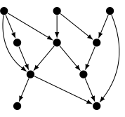
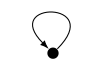
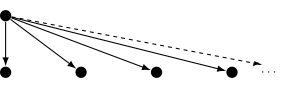
For example, Figure 3 and Figure 4 are games, but Figure 5, Figure 6, and Figure 7 are not games.

Diagram
Figure 3. An example of a finite game
⋯
Figure 4. An example of an infinite game
Diagram
Figure 5. An example of non-game with infinite path
⋯; ⋯
Figure 6. Another example of non-game with infinite path
⋯
Figure 7. An example of non-game with infinite options

The ultimate goal of combinatorial game theory is to win a given game. To win a game is almost the same thing as knowing outcome, “NN-states” (Next-player-winning states) or “PP-states” (Previous-player-winning states), defined as follows.

Definition 2.2 (Outcome).

For a game 𝕏=(X,→)\mathbb{X}=(X,\to) and its state x∈Xx\in X, the outcome of xx is defined by

𝖮𝗎𝗍𝖼𝗈𝗆𝖾𝕏​(x)≔{N(if the next player wins from the state x)P(if the previous player wins from the state x),\mathsf{Outcome}_{\mathbb{X}}(x)\coloneqq\begin{cases}N&\textrm{(if the next player wins from the state $x$)}\\ P&\textrm{(if the previous player wins from the state $x$),}\end{cases}

or equivalently, it is recursively defined by

𝖮𝗎𝗍𝖼𝗈𝗆𝖾𝕏​(x)≔{N(if there exists x→x′ with 𝖮𝗎𝗍𝖼𝗈𝗆𝖾𝕏​(x′)=P)P(otherwise)\mathsf{Outcome}_{\mathbb{X}}(x)\coloneqq\begin{cases}N&\textrm{(if there exists $x\to x^{\prime}$ with $\mathsf{Outcome}_{\mathbb{X}}(x^{\prime})=P$)}\\ P&\textrm{(otherwise)}\end{cases}

The latter recursive definition is not circuler, thanks to the “finite time” condition.

Remark 2.3 (How can we win with outcome?).

For those who are not familiar with combinatorial game theory, let us clarify the connection between an actual ways to win a game 𝕏=(X,→)\mathbb{X}=(X,{\to}) and the outcome function 𝖮𝗎𝗍𝖼𝗈𝗆𝖾:X→{N,P}\mathsf{Outcome}\colon X\to\{N,P\}. Suppose it is your turn and the current position is an NN-state. Then the winning strategy is simply to always move to a PP-state. By the definition of PP-states, your opponent cannot reply with another PP-state. The opponent must either move to an NN-state, or lose immediately. In the latter case, by the definition of NN-states, you can move to a PP-state again. Due to the finite time condition, this procedure must terminate, and therefore you are guaranteed to win.

Remark 2.4 (Why do we assume the “finite options” condition?).

While we do not assume the finiteness of the underlying set, we include the “finite options” condition in Definition 2.1. This kind of “local finiteness” condition is a difference with [Baš+24] and a similarity with [DG24]. We assume it not only because many games of interest satisfy the condition, but also we need it in the following sections. Let us explain some (of many) reasons why we need it. One game theoretic reason is that it is necessary to define the Grundy number while dealing with games with infinite states. (More precisely, we need it to keep Grundy number to be finite ordinal.) A categorical reason is that the considered functor 𝒫fin:𝐒𝐞𝐭→𝐒𝐞𝐭\mathcal{P}_{\mathrm{fin}}\colon\mathbf{Set}\to\mathbf{Set} is finitary ([ALM07, Example 2.5, Example 3.18]) and hence our category of games admits a lot of pleasant properties (Appendix B). In particular, thanks to the finite option condition, we have the terminal game (Proposition 3.31), which plays the central role in our characterization of nim-sum.

Example 2.5 (Winning strategy of the subtraction nim).

Let us give a famous example of the outcome function. A subtraction nim (for S={1,2,3}S=\{1,2,3\}) is (ℕ,→)(\mathbb{N},{\to}), where

n→m⇔n=m+1,m+2,or ​m+3.n\to m\iff n=m+1,m+2,\textrm{or }m+3.

We can (recursively) prove that the outcome function is given by

𝖮𝗎𝗍𝖼𝗈𝗆𝖾⁡(n)={N(n≢0mod4)P(n≡0mod4).\mathsf{Outcome}(n)=\begin{cases}N&(n\not\equiv 0\mod 4)\\ P&(n\equiv 0\mod 4).\end{cases}

So the winning strategy is to move to the multiples of 44.

Theoretically, the most important game might be the following game, which we will call the binary exponent nim, or later, the terminal game (Remark 3.33).

Example 2.6 (Binary exponent nim, or the terminal game).

The underlying set of the binary exponent nim is ℕ\mathbb{N}, and the relation n→mn\to m is defined by

n→m⇔2m​ appears in the binary expansion of ​n.n\to m\iff 2^{m}\textrm{ appears in the binary expansion of }n.

For example, when n=10000n=10000, since

n=10000=213+210+29+28+24,n=10000=2^{13}+2^{10}+2^{9}+2^{8}+2^{4},

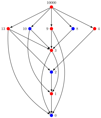
there are 55 possible moves, namely 10000→4,8,9,10,1310000\to 4,8,9,10,13. The state n=10000n=10000 is NN-state, and the winning way it to move to 88 or 1010 (Figure 8).

Diagram
Figure 8. The binary exponent nim, below 1000010000, with PP-states and NN-states.
Example 2.7 (“Effeuiller la marguerite”).

Let us consider another game whose underlying set is ℕ\mathbb{N}. This time, we define n→mn\to m by

n→m⇔n=m+1.n\to m\iff n=m+1.

In each phase, players have at most one option. Obviously, the outcome of a state nn of this boring game is determined only by the parity of nn; a state nn is a PP-state if and only if nn is even. We will write ElM\mathrm{ElM} for this game since this game is conventionally called “effeuiller la marguerite.” Althogh this game ElM=(ℕ,−1)\mathrm{ElM}=(\mathbb{N},-1) is practically quite boring, it sometimes plays a theoretical role (Example 4.16, Example C.3).

We conclude this subsection by expressing Bouton’s theorem in our formulation (Definition 2.1) as follows.

Example 2.8 (Nim).

In our formulation, the nn-heap nim Nimn\mathrm{Nim}_{n} is (ℕn,→)(\mathbb{N}^{n},\to), where (a1,…​an)→(b1,…​bn)(a_{1},\dots a_{n})\to(b_{1},\dots b_{n}) is defined by

(a1,…​an)→(b1,…​bn)⇔there exists 1≤i≤n such that ai>bi and for any j≠i, aj=bj(a_{1},\dots a_{n})\to(b_{1},\dots b_{n})\iff\textrm{there exists $1\leq i\leq n$ such that $a_{i}>b_{i}$ and for any $j\neq i$, $a_{j}=b_{j}$}
Theorem 2.9 (Bouton’s theorem [Bou01]).

A state (a1,…,an)(a_{1},\dots,a_{n}) of the nn-heap nim Nimn\mathrm{Nim}_{n} is PP-state if and only if a1⊕⋯⊕an=0a_{1}\oplus\cdots\oplus a_{n}=0.

2.2. Divide difficulties with the Conway addition and Grundy number

In the last subsection, we have seen that once you know the outcome of a given game, you know the winning strategy. But how can we effectively calculate the outcome? (For example, how can we know that the outcome of a nim state (a1,…,an)(a_{1},\dots,a_{n}) is PP if and only if a1⊕⋯⊕an=0a_{1}\oplus\dots\oplus a_{n}=0?)

One promising strategy is to divide the difficulty into smaller parts! What we will do in this subsection (and the whole Section 4) is to decompose a game into smaller parts and synthesize the properties of smaller games:

  • •

    We want to know the outcome of a game 𝕏\mathbb{X}.

  • •

    We devide the game 𝕏\mathbb{X} into a Conway sum (Definition 2.10) of smaller games 𝕏=𝕐+ℤ\mathbb{X}=\mathbb{Y}+\mathbb{Z}.

  • •

    We calculate the Grundy numbers (Definition 2.14) of the games 𝕐,ℤ\mathbb{Y},\mathbb{Z}.

  • •

    We calculate the Grundy numbers of 𝕏\mathbb{X} from those of 𝕐,ℤ\mathbb{Y},\mathbb{Z} (Theorem 2.17).

  • •

    We calculate the outcome of 𝕏\mathbb{X} from the Grundy number of 𝕏\mathbb{X} (Proposition 2.15).

Let us clarify again that all the content in this subsection is well-known in combinatorial game theory. For more details, see standard textbooks including [Sie13].

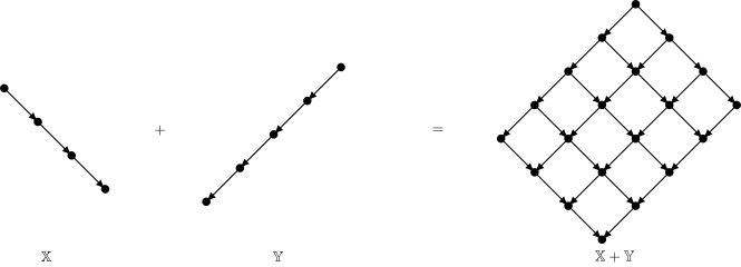
First, we recall the notion of the Conway addition of games, which is visualized in Figure 9.

Definition 2.10 (Conway addition of games).

For two games 𝕏=(X,→𝕏),𝕐=(Y,→𝕐)\mathbb{X}=(X,\to_{\mathbb{X}}),\mathbb{Y}=(Y,\to_{\mathbb{Y}}), their Conway sum (or just sum) 𝕏+𝕐\mathbb{X}+\mathbb{Y} is the game (X×Y,→𝕏+𝕐)(X\times Y,\to_{\mathbb{X}+\mathbb{Y}}), where (x,y)→𝕏+𝕐(x′,y′)(x,y)\to_{\mathbb{X}+\mathbb{Y}}(x^{\prime},y^{\prime}) if and only if (x→𝕏x′∧y=y′)(x\to_{\mathbb{X}}x^{\prime}\land y=y^{\prime}) or (x=x′∧y→𝕐y′)(x=x^{\prime}\land y\to_{\mathbb{Y}}y^{\prime}).

𝕏; +; 𝕐; =; 𝕏+𝕐
Figure 9. An example of Conway addition.
Remark 2.11 (Terminology and notation: Why is it called “sum”?).

The Conway sum is conventionally called “sum” and denoted by 𝕏+𝕐\mathbb{X}+\mathbb{Y}, while some readers might think “product” is a better name. In fact, the corresponding monoidal structure in graph theory is called the box “product” (see, for example, [KK24], which is also related to Section 5.3). But there is a decent reason to call it “sum” in game theory, related to the surreal number [Con00].

A typical usage of the Conway addition is to decompose a complicated game into smaller games. The prototypical example is the following decomposition of nim.

Example 2.12 (Decomposition of Nim).

The nn-heaps nim Nimn\mathrm{Nim}_{n} is the Conway sum of nn-copies of (11-heap) nim games.

Nimn=Nim1+⋯+Nim1\mathrm{Nim}_{n}=\mathrm{Nim}_{1}+\dots+\mathrm{Nim}_{1}

We want to utilize the Conway addition ++ to calculate the outcome of a state (x,y)∈𝕏+𝕐(x,y)\in\mathbb{X}+\mathbb{Y}. However, even if you know the outcomes 𝖮𝗎𝗍𝖼𝗈𝗆𝖾𝕏​(x)\mathsf{Outcome}_{\mathbb{X}}(x) and 𝖮𝗎𝗍𝖼𝗈𝗆𝖾𝕐​(y)\mathsf{Outcome}_{\mathbb{Y}}(y), it is generally impossible to calculate the outcome of the sum state 𝖮𝗎𝗍𝖼𝗈𝗆𝖾𝕏+𝕐​(x,y)\mathsf{Outcome}_{\mathbb{X}+\mathbb{Y}}(x,y). Thus we need to enrich the outcome into the Grundy number. As a preparation, we recall the notion of mex, which stands for minimum excluded value.

Definition 2.13 (mex).

For a finite set of natural numbers S⊂ℕS\subset\mathbb{N}, its mex, denoted by 𝗆𝖾𝗑⁡(S)∈ℕ\mathsf{mex}(S)\in\mathbb{N}, is the minimum natural number that does not belong to the subset SS. In other words, mex of SS is the minimum element of the complement of SS:

𝗆𝖾𝗑⁡(S)=min⁡Sc.\mathsf{mex}(S)=\min S^{\mathrm{c}}.

Notice that the complement ScS^{c} is always non-empty since the set SS is assumed to be finite (cf. Remark 2.4).

Definition 2.14 (Grundy number).

For a game 𝕏=(X,→)\mathbb{X}=(X,\to) and a state x∈Xx\in X, its Grundy number 𝖦𝗋𝗎𝗇𝖽𝗒𝕏​(x)\mathsf{Grundy}_{\mathbb{X}}(x) is recursively defined by

(1) 𝖦𝗋𝗎𝗇𝖽𝗒𝕏​(x)≔𝗆𝖾𝗑⁡({𝖦𝗋𝗎𝗇𝖽𝗒𝕏​(x′)∣x→x′}).\mathsf{Grundy}_{\mathbb{X}}(x)\coloneqq\mathsf{mex}(\{\mathsf{Grundy}_{\mathbb{X}}(x^{\prime})\mid x\to x^{\prime}\}).

This recursive definition does work due to the two finiteness conditions in the definition of games (Definition 2.1). See Figure 10 for an example of a recursive calculation of the Grundy numbers.
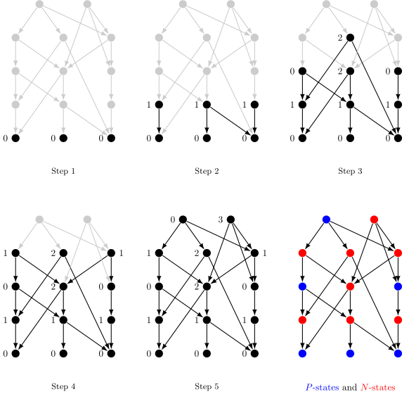
0; 0; 0; 0; 0; 0; 1; 1; 1; 0; 0; 0; 1; 1; 1; 0; 2; 0; 2; 0; 0; 0; 1; 1; 1; 0; 2; 0; 1; 2; 1; 0; 0; 0; 1; 1; 1; 0; 2; 0; 1; 2; 1; 0; 3; P; N
Figure 10. Recursive calculation of Grundy numbers from bottom to top, and the outcome

The importance of the Grundy number is due to the following proposition.

Proposition 2.15 (the Grundy number is more informative than the outcome).

For any game 𝕏=(X,→)\mathbb{X}=(X,{\to}) and any state x∈Xx\in X, its outcome is PP if and only if its Grundy number 𝖦𝗋𝗎𝗇𝖽𝗒𝕏​(x)\mathsf{Grundy}_{\mathbb{X}}(x) is 00:

𝖮𝗎𝗍𝖼𝗈𝗆𝖾𝕏​(x)=P⇔𝖦𝗋𝗎𝗇𝖽𝗒𝕏​(x)=0.\mathsf{Outcome}_{\mathbb{X}}(x)=P\iff\mathsf{Grundy}_{\mathbb{X}}(x)=0.
Proof.

One can easily prove this by induction, although we will see more conceptual proof later (Proposition 3.26). ∎

The reason why we enrich the ouctome to Grundy number is that the Grundy number is compatible with the Conway addition (Theorem 2.17)! Let us recall nim-sum again (Definition 1.1).

Definition 2.16 (Nim-sum).

The nim-sum is the abelian group structure on ℕ\mathbb{N}, induced by the bijection ℕ→⨁k=0∞ℤ/2​ℤ\mathbb{N}\to\bigoplus_{k=0}^{\infty}\mathbb{Z}/2\mathbb{Z} given by the binary expansion. In other words, the nim-sum is the digit-wise exclusive disjunction (xor) of the binary expansion.

For example, 7⊕5=(111)2⊕(101)2=(010)2=27\oplus 5=(111)_{2}\oplus(101)_{2}=(010)_{2}=2.

Theorem 2.17 (Nim-sum rule= generalized Bouton’s theorem [Sie13, II. Theorem4.7]).

For any pair of games 𝕏=(X,→𝕏),𝕐=(Y,→𝕐)\mathbb{X}=(X,\to_{\mathbb{X}}),\mathbb{Y}=(Y,\to_{\mathbb{Y}}) and any pair of states x∈Xx\in X, y∈Yy\in Y, the Grundy number of (x,y)(x,y) is given by the nim-sum as follows:

𝖦𝗋𝗎𝗇𝖽𝗒𝕏+𝕐​(x,y)=𝖦𝗋𝗎𝗇𝖽𝗒𝕏​(x)⊕𝖦𝗋𝗎𝗇𝖽𝗒𝕐​(y).\mathsf{Grundy}_{\mathbb{X}+\mathbb{Y}}(x,y)=\mathsf{Grundy}_{\mathbb{X}}(x)\oplus\mathsf{Grundy}_{\mathbb{Y}}(y).

Combining Proposition 2.15 and Theorem 2.17, we can calculate PP-states of a Conway sum and thus its winning strategy. In fact, for a given game 𝕏\mathbb{X} that can be decomposed into a Conway sum of two games 𝕏=𝕐+ℤ\mathbb{X}=\mathbb{Y}+\mathbb{Z}, we have

x=(y,z)​ is a P-state⇔𝖦𝗋𝗎𝗇𝖽𝗒𝕐+ℤ​(y,z)=0⇔𝖦𝗋𝗎𝗇𝖽𝗒𝕐​(y)⊕𝖦𝗋𝗎𝗇𝖽𝗒ℤ​(z)=0.x=(y,z)\textrm{ is a $P$-state}{\iff}\mathsf{Grundy}_{\mathbb{Y}+\mathbb{Z}}(y,z)=0\iff\mathsf{Grundy}_{\mathbb{Y}}(y)\oplus\mathsf{Grundy}_{\mathbb{Z}}(z)=0.
Example 2.18 (Analysis of nim).

The classical Bouton theorem (Theorem 2.9) is the typical example of the above observation. As the nn-heap nim Nimn\mathrm{Nim}_{n} is the Conway sum of nn-copies of the 11-heap nim Nim1\mathrm{Nim}_{1} (Example 2.12), in order to win Nimn\mathrm{Nim}_{n}, it suffices to know 𝖦𝗋𝗎𝗇𝖽𝗒Nim1:ℕ→ℕ\mathsf{Grundy}_{\mathrm{Nim}_{1}}\colon\mathbb{N}\to\mathbb{N}. By the easy induction, we can prove that 𝖦𝗋𝗎𝗇𝖽𝗒Nim1=idℕ\mathsf{Grundy}_{\mathrm{Nim}_{1}}=\mathrm{id}_{\mathbb{N}} (cf. Appendix C), and thus we obtain

𝖦𝗋𝗎𝗇𝖽𝗒Nimn​(a1,…,an)=𝖦𝗋𝗎𝗇𝖽𝗒Nim1​(a1)⊕⋯⊕𝖦𝗋𝗎𝗇𝖽𝗒Nim1​(an)=a1⊕⋯⊕an.\mathsf{Grundy}_{\mathrm{Nim}_{n}}(a_{1},\dots,a_{n})=\mathsf{Grundy}_{\mathrm{Nim}_{1}}(a_{1})\oplus\dots\oplus\mathsf{Grundy}_{\mathrm{Nim}_{1}}(a_{n})=a_{1}\oplus\dots\oplus a_{n}.

Therefore, Proposition 2.15 implies that a state (a1,…,an)(a_{1},\dots,a_{n}) is a PP-state if and only if a1⊕⋯⊕an=0a_{1}\oplus\dots\oplus a_{n}=0, which is exactly what the Bouton theorem states (Theorem 2.9).

3. Games as recursive coalgebras

In this section and the next section, we will reinterpret the content in Section 2 in terms of recursive coalgebras. Here is the spoiler:

Abstract Coalgebra Theory Game Theoretic Notions example
Recursive coalgebra section 3.3 Game Nim\mathrm{Nim}
Coalgebra homomorphism section 3.4 Game morphism
Algebra section 3.5 recursion step of game value mex
Algebra homomorphism section 3.5 Transformation of game value Proposition 2.15
Coalgebra-algebra morphism section 3.5 Game value Grundy number
Terminal recursive coalgebra section 3.6 Binary exponent nim
Monoidal structure section 4.1 Game decomposition Conway sum
Bouton monoid section 4.2 Nim-sum
Table 1. Comparison between coalgebra theory and game theory

Before delving into the reinterpretation part, we first observe a motivating phenomenon in Section 3.1, and recall the theory of recursive coalgebras in Section 3.2.

3.1. Why recursive coalgebras?

Before explaining the categorical abstract nonsense in Section 3.2, let us observe one phenomenon motivating the latter contents. The reader can skip this subsection since it does not include any theorems. However, we recommend to read it because this observation is the starting idea of this project44 4 This observation can be found also in [Baš+24, section 4], which does not use coalgebra theory..

Our original motivation is to understand the nim-sum (Definition 2.16), and the reason why the nim-sum works is the Nim-sum rule (Theorem 2.17) regarding the Grundy number (Definition 2.14). So our first task would be to understand the Grundy number categorically.

In the definition of Grundy number, we used a particular type of recursion

𝖦𝗋𝗎𝗇𝖽𝗒𝕏​(x)=𝗆𝖾𝗑⁡({𝖦𝗋𝗎𝗇𝖽𝗒𝕏​(x′)∣x→x′})​ (1).\mathsf{Grundy}_{\mathbb{X}}(x)=\mathsf{mex}(\{\mathsf{Grundy}_{\mathbb{X}}(x^{\prime})\mid x\to x^{\prime}\})\text{ (\ref{eq:GrundyNumber})}.

Let 𝒫fin​(X)\mathcal{P}_{\mathrm{fin}}(X) denote the set of all finite subset of a given set XX (Notation 3.9). Then, the mex function is a function from 𝒫fin​(ℕ)\mathcal{P}_{\mathrm{fin}}(\mathbb{N}) to ℕ\mathbb{N}:

𝗆𝖾𝗑:𝒫fin​(ℕ)→ℕ.\mathsf{mex}\colon\mathcal{P}_{\mathrm{fin}}(\mathbb{N})\to\mathbb{N}.

Similarly, we can rewrite games as a function between 𝒫fin​(X)\mathcal{P}_{\mathrm{fin}}(X) and XX, but in the opposite direction! For any directed graph (X,→⊂X×X)(X,{\to}\subset X\times X), the corresponding neighborhood function θ:X→𝒫⁡(X)\theta\colon X\to\mathcal{P}(X) is defined by

(2) θ⁡(x)={x′∈X∣x→x′}.\theta(x)=\{x^{\prime}\in X\mid x\to x^{\prime}\}.

If a graph 𝕏=(X,→)\mathbb{X}=(X,{\to}) satisfies the finite option condition in Definition 2.1, in particular, if 𝕏\mathbb{X} is a game, the codomain 𝒫⁡(X)\mathcal{P}(X) can be reduced to 𝒫fin​(X)\mathcal{P}_{\mathrm{fin}}(X) and we obtain the function

θ:X→𝒫fin​(X).\theta\colon X\to\mathcal{P}_{\mathrm{fin}}(X).

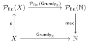
Thus, we can rephrase the definition of Grundy number (Definition 2.14 and Equation 1) as the unique function 𝖦𝗋𝗎𝗇𝖽𝗒𝕏:X→ℕ\mathsf{Grundy}_{\mathbb{X}}\colon X\to\mathbb{N} that makes the following “twisted” diagram

(3) 𝒫fin(X); 𝒫fin(ℕ); X; ℕ; 𝒫fin(𝖦𝗋𝗎𝗇𝖽𝗒𝕏); 𝗆𝖾𝗑; θ; 𝖦𝗋𝗎𝗇𝖽𝗒𝕏

commutative, where 𝒫fin​(𝖦𝗋𝗎𝗇𝖽𝗒𝕏)\mathcal{P}_{\mathrm{fin}}(\mathsf{Grundy}_{\mathbb{X}}) denotes the direct image function! The “finite time” condition ensures the unique existence of such a function 𝖦𝗋𝗎𝗇𝖽𝗒𝕏:X→A\mathsf{Grundy}_{\mathbb{X}}\colon X\to A.

One may find it weird to consider such a twisted diagram. However this reflects a kind of “twistedness” of the computation of the Grundy number; the recursive computation of Grundy numbers, as in Figure 10, is carried out by tracing the game backwards. The somewhat unusual kind of “twisted” commutativity in Diagram 3 corresponds to the nature of this recursive computation that goes against the flow of the game! Such “twisted recursive computations” have a long history in category theory (or categorical computer science) under the name of recursive coalgebras (or hylomorphisms), which we will recall in the next subsection.

3.2. Preliminaries on coalgebras and recursive coalgebras

This subsection aims to recall the basic notions in coalgebra theory, in particular, the definition and properties of recursive coalgebras. The reades are assumed to be familiar with the definitions of categories and functors, (and limits for Section 3.6). For example, the first three sections of [Mac98] suffice. For general theory and examples of coalgebras, see [Jac17]. For recursive coalgebras, see the book [Tay99], papers including [AMM20], or papers cited therein.

In order to separate the general theory from our particular context of game theory, we intentionally postpone the motivating examples untill the next subsection. So if the reader feels that it is too abstract, please refer to the next section for our game-theoretic examples.

3.2.1. Algebras and coalgebras of an endofunctor

The definition of coalgebras (and algebras) of an endofunctor is surprisingly simple:

Definition 3.1 (Coalgebras and algebras).

For an endofunctor T:𝒞→𝒞T\colon\mathcal{C}\to\mathcal{C} on a category 𝒞\mathcal{C}, a TT-coalgebra 𝕏\mathbb{X} is a pair 𝕏=(X,θ)\mathbb{X}=(X,\theta) of an object X∈ob⁡(𝒞)X\in\mathrm{ob}(\mathcal{C}) and a morphism θ:X→T​X\theta\colon X\to TX. Dually, a TT-algebra 𝔸\mathbb{A} is a pair 𝔸=(A,α)\mathbb{A}=(A,\alpha) of an object A∈ob⁡(𝒞)A\in\mathrm{ob}(\mathcal{C}) and a morphism α:T​A→A\alpha\colon TA\to A.

Definition 3.2 (Coalgebra homomorphism and algebra homomorphism).

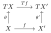
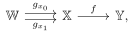
For an endofunctor T:𝒞→𝒞T\colon\mathcal{C}\to\mathcal{C} on a category 𝒞\mathcal{C}, a homomorphism of TT-coalgebras from (X,θ)(X,\theta) to (X′,θ′)(X^{\prime},\theta^{\prime}) is a morphism f:X→X′f\colon X\to X^{\prime} in 𝒞\mathcal{C} such that the diagram

TX; TX′; X; X′; Tf; f; θ; θ′

commutes. Homomorohisms between TT-algebras (A,α),(A′,α′)(A,\alpha),(A^{\prime},\alpha^{\prime}) are defined in the dual way:

TA; TA′; A; A′.; Tf; α; α′; f
Notation 3.3.

For an endofunctor T:𝒞→𝒞T\colon\mathcal{C}\to\mathcal{C} on a category 𝒞\mathcal{C}, the category of TT-coalgebras and TT-coalgebra homomorphisms is denoted by 𝐂𝐨𝐚𝐥𝐠T\mathbf{Coalg}_{T}. The category of TT-algebras and TT-algebra homomorphisms is denoted by 𝐀𝐥𝐠T\mathbf{Alg}_{T}.

3.2.2. Coalgebra-algebra morphisms and Recursive coalgebras

We will recall the notion of recursive coalgebra, due to [Osi74] and [Tay99].

Definition 3.4.

For an endofunctor T:𝒞→𝒞T\colon\mathcal{C}\to\mathcal{C} on a category 𝒞\mathcal{C}, a coalgebra-algebra morphism from a TT-coalgebra 𝕏=(X,θ)\mathbb{X}=(X,\theta) to a TT-algebra 𝔸=(A,α)\mathbb{A}=(A,\alpha) is a morphism f:X→Af\colon X\to A in the category 𝒞\mathcal{C} such that the diagram

TX; TA; X; A; Tf; α; θ; f

commutes.

Definition 3.5 (Recursive coalgebra).

A TT-coalgebra 𝕏=(X,θ)\mathbb{X}=(X,\theta) is said to be recursive if, for any TT-alegebra 𝔸=(A,α)\mathbb{A}=(A,\alpha), there exists a unique coalgebra-algebra morphism from 𝕏\mathbb{X} to 𝔸\mathbb{A}. The full subcategory of 𝐂𝐨𝐚𝐥𝐠T\mathbf{Coalg}_{T} that consists of all recursive TT-coalgebras is denoted by 𝐑𝐞𝐜𝐂𝐨𝐚𝐥𝐠T\mathbf{RecCoalg}_{T}.

For a recursive coalgebra 𝕏=(X,θ)\mathbb{X}=(X,\theta) and a TT-algebra 𝔸=(A,α)\mathbb{A}=(A,\alpha), the unique coalgebra-algebra morphism X→AX\to A is called the hylomorphism and denoted by 𝗁𝗒𝗅𝗈𝔸,𝕏:X→A\mathsf{hylo}_{\mathbb{A},\mathbb{X}}\colon X\to A.

Let us emphasize the following “stability” of hylomorphisms by compositions, which is theoretically almost trivial, but it provides a seemingly non-trivial consequences including Proposition 3.18, Corollary 3.25, and Proposition 3.26, which generalizes Proposition 2.15.

Lemma 3.6 (Stability of hylomorphisms by composition).

Let T:𝒞→𝒞T\colon\mathcal{C}\to\mathcal{C} be an endofunctor on a category 𝒞\mathcal{C}, 𝕏=(X,θ)\mathbb{X}=(X,\theta) be a recursive TT-coalgebra, 𝔸=(A,α)\mathbb{A}=(A,\alpha) be a TT-algebra, and 𝗁𝗒𝗅𝗈𝔸,𝕏:X→A\mathsf{hylo}_{\mathbb{A},\mathbb{X}}\colon X\to A be the hylomorphism between them.

  • •

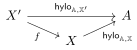
    For any recurisive TT-coalgebra 𝕏′=(X′,θ′)\mathbb{X}^{\prime}=(X^{\prime},\theta^{\prime}) and any TT-coalgebra homomorphism f:𝕏′→𝕏f\colon\mathbb{X}^{\prime}\to\mathbb{X}, the hylomorphism 𝗁𝗒𝗅𝗈𝔸,𝕏′:X′→A\mathsf{hylo}_{\mathbb{A},\mathbb{X}^{\prime}}\colon X^{\prime}\to A is given by 𝗁𝗒𝗅𝗈𝔸,𝕏′=𝗁𝗒𝗅𝗈𝔸,𝕏∘f\mathsf{hylo}_{\mathbb{A},\mathbb{X}^{\prime}}=\mathsf{hylo}_{\mathbb{A},\mathbb{X}}\circ f.

    X′; A; X; 𝗁𝗒𝗅𝗈𝔸,𝕏′; f; 𝗁𝗒𝗅𝗈𝔸,𝕏
  • •

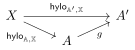
    For any TT-algebra 𝔸′=(A′,α′)\mathbb{A}^{\prime}=(A^{\prime},\alpha^{\prime}) and any TT-algebra homomorphism g:𝔸→𝔸′g\colon\mathbb{A}\to\mathbb{A}^{\prime}, the hylomorphism 𝗁𝗒𝗅𝗈𝔸′,𝕏:X→A′\mathsf{hylo}_{\mathbb{A}^{\prime},\mathbb{X}}\colon X\to A^{\prime} is given by 𝗁𝗒𝗅𝗈𝔸′,𝕏=g∘𝗁𝗒𝗅𝗈𝔸,𝕏\mathsf{hylo}_{\mathbb{A}^{\prime},\mathbb{X}}=g\circ\mathsf{hylo}_{\mathbb{A},\mathbb{X}}.

    X; A′; A; 𝗁𝗒𝗅𝗈𝔸′,𝕏; 𝗁𝗒𝗅𝗈𝔸,𝕏; g
Proof.

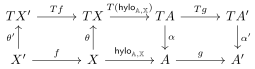
The commutative diagmram

TX′; TX; TA; TA′; X′; X; A; A′; Tf; T⁡(𝗁𝗒𝗅𝗈𝔸,𝕏); Tg; α; α′; f; θ′; θ; 𝗁𝗒𝗅𝗈𝔸,𝕏; g

completes the proof. ∎

As we are interested in the terminal object of 𝐑𝐞𝐜𝐂𝐨𝐚𝐥𝐠T\mathbf{RecCoalg}_{T}, let us recall the related result from [Lam68] and [CUV06].

Proposition 3.7 (Initial algebra is the terminal recursive coalgebra).

For an endofunctor T:𝒞→𝒞T\colon\mathcal{C}\to\mathcal{C} on a category 𝒞\mathcal{C}, if a TT-algebra 𝔸=(A,α)\mathbb{A}=(A,\alpha) is the initial TT-algebra, then

  • •

    the structure map α:T​A→A\alpha\colon TA\to A is an isomorphism [Lam68, Lemma 2.2], and

  • •

    the coalgebra (A,α−1:A→TA)(A,\alpha^{-1}\colon A\to TA) is the terminal recursive coalgebra [CUV06, Proposition 2].

Proof.

Both are easily checked by diagram chases. The first assertion is known as Lambek’s lemma. ∎

Remark 3.8 (Relationship with well-founded coalgebras).

Actually, the recursive coalgebras we will consider (Section 3.3) are also characterized as well-founed coalgebras, which are known to be inherently related to recursice coalgebras. For their relationships, see [Tay99] and also a recent study [AMM20].

3.3. Games as recursive 𝒫fin\mathcal{P}_{\mathrm{fin}}-coalgebras

In the rest of Section 3, we will specialize the general theory of recursive coalgebra (Section 3.2) to the case where the endofunctor T:𝒞→𝒞T\colon\mathcal{C}\to\mathcal{C} is the the finite powerset functor.

Notation 3.9 (finite powerset functor).

In this paper,

  • •

    𝒫:𝐒𝐞𝐭→𝐒𝐞𝐭\mathcal{P}\colon\mathbf{Set}\to\mathbf{Set} denotes the covariant powerset functor that sends a set to its powerset and a function to its direct image function, and

  • •

    𝒫fin:𝐒𝐞𝐭→𝐒𝐞𝐭\mathcal{P}_{\mathrm{fin}}:\mathbf{Set}\to\mathbf{Set} denotes the finite powerset functor, which is the subfunctor of 𝒫:𝐒𝐞𝐭→𝐒𝐞𝐭\mathcal{P}:\mathbf{Set}\to\mathbf{Set} such that 𝒫fin​(X)={S⊂X∣#​S<∞}\mathcal{P}_{\mathrm{fin}}(X)=\{S\subset X\mid\#S<\infty\}.

In terms of coalgebras, any graph 𝕏=(X,→)\mathbb{X}=(X,{\to}) is associated with the corresponding 𝒫\mathcal{P}-coalgebra

θ:X→𝒫⁡(X)\theta\colon X\to\mathcal{P}(X)

by Equation 2. The finite option condition in Definition 2.1 is precisely saying that the codomain 𝒫⁡(X)\mathcal{P}(X) can be reduced to 𝒫fin​(X)\mathcal{P}_{\mathrm{fin}}(X). The next proposition states that the finite time condition is precicely the recursiveness (Definition 3.5) and characterize games as the graphs that admits the “twisted recursion” (Diagram 3).

Proposition 3.10 (Games as recursive coalgebras).

For any graph 𝕏=(X,→)\mathbb{X}=(X,{\to}) with the finite option condition (Definition 2.1), the corresponding 𝒫fin\mathcal{P}_{\mathrm{fin}}-coalgebra

θ:X→𝒫fin​(X)\theta\colon X\to\mathcal{P}_{\mathrm{fin}}(X)

is a recursive coalgebra if and only if 𝕏\mathbb{X} is a game. In particular, for any set XX, Equation 2 provides a one-to-one correspondence between the game structures on XX and the recursive 𝒫fin\mathcal{P}_{\mathrm{fin}}-coalgebra structures on XX.

Proof.

Let 𝕏=(X,→)\mathbb{X}=(X,{\to}) be a graph with the finite option condition. If the graph is a game, i.e., satisfies the finite time condition, we can recursively construct the unique coalgebra-algebra morphism to any 𝒫fin\mathcal{P}_{\mathrm{fin}}-algebra, and hence we can prove that it is a recursive coalgebra.

Conversely, take an arbitrary recursive coalgebra 𝕏=(X,θ)\mathbb{X}=(X,\theta). We prove that the corresponding graph (X,→)(X,\to) satisfies the finite time condition. Consider a 𝒫fin\mathcal{P}_{\mathrm{fin}}-algebra 𝔸=({⊤,⊥},α)\mathbb{A}=(\{\top,\bot\},\alpha) defined by

α⁡(S)≔{⊤(⊥∉S)⊥(⊥∈S).\alpha(S)\coloneqq\begin{cases}\top&(\bot\notin S)\\ \bot&(\bot\in S).\end{cases}

On the one hand, the function 𝖥𝗂𝗇𝖳𝗂𝗆𝖾𝕏:X→{⊤,⊥}\mathsf{FinTime}_{\mathbb{X}}\colon X\to\{\top,\bot\} defined by

𝖥𝗂𝗇𝖳𝗂𝗆𝖾𝕏​(x)≔{⊤(any path starting from x terminates in finite steps)⊥(otherwise)\mathsf{FinTime}_{\mathbb{X}}(x)\coloneqq\begin{cases}\top&(\textrm{any path starting from $x$ terminates in finite steps})\\ \bot&(\textrm{otherwise})\end{cases}

is an coalgebra-algebra morphism from 𝕏\mathbb{X} to 𝔸\mathbb{A}. On the other hand, the constant function to ⊤\top, which is denoted by 𝖳𝗋𝗎𝖾𝕏:X→{⊤,⊥}\mathsf{True}_{\mathbb{X}}\colon X\to\{\top,\bot\}, is also a coalgebra-algebra morphism from 𝕏\mathbb{X} to 𝔸\mathbb{A}. Therefore, the assumption that 𝕏\mathbb{X} is recursive implies that 𝖥𝗂𝗇𝖳𝗂𝗆𝖾𝕏=𝖳𝗋𝗎𝖾𝕏\mathsf{FinTime}_{\mathbb{X}}=\mathsf{True}_{\mathbb{X}}, i.e., 𝕏\mathbb{X} satisfies the finite time condition. ∎

Example 3.11 (Nim as a recursive coalgebra).

Let (ℕ,ν:ℕ→𝒫fin(ℕ))(\mathbb{N},\nu\colon\mathbb{N}\to\mathcal{P}_{\mathrm{fin}}(\mathbb{N})) denote the 𝒫fin\mathcal{P}_{\mathrm{fin}}-coalgebra corresponding to the (11-heap) nim game Nim1\mathrm{Nim}_{1} (Example 2.8). This function ν:ℕ→𝒫fin​(ℕ)\nu\colon\mathbb{N}\to\mathcal{P}_{\mathrm{fin}}(\mathbb{N}) is given by

μ⁡(n)={0,1,…,n−1},\mu(n)=\{0,1,\dots,n-1\},

which looks like the von Neumann set-theoretic definition of natural numbers. This analogy becomes more precise in Example 3.35.

3.4. Game morphisms as 𝒫fin\mathcal{P}_{\mathrm{fin}}-coalgebra homomorphismsm

As games are recursive coalgebras, it is reasonable to define game morphisms as coalgebra homomorphisms. Notice that being a coalgebra homomorphism is much stronger than just being a graph morphism! For games 𝕏=(X,→𝕏)\mathbb{X}=(X,{\to_{\mathbb{X}}}) and 𝕐=(Y,→𝕐)\mathbb{Y}=(Y,{\to_{\mathbb{Y}}}) and a function f:X→Yf\colon X\to Y, being a graph morphism x0→x1⟹f⁡(x0)→f⁡(x1)x_{0}\to x_{1}\implies f(x_{0})\to f(x_{1}) is equivalent to saying that f⁡(θ𝕏​(x))⊂θ𝕐​(f⁡(x))f(\theta_{\mathbb{X}}(x))\subset\theta_{\mathbb{Y}}(f(x)), which is strictly weaker than being a coalgebra homomorphism f⁡(θ𝕏​(x))=θ𝕐​(f⁡(x))f(\theta_{\mathbb{X}}(x))=\theta_{\mathbb{Y}}(f(x)). In order to ensure the opposite inclusion f⁡(θ𝕏​(x))⊃θ𝕐​(f⁡(x))f(\theta_{\mathbb{X}}(x))\supset\theta_{\mathbb{Y}}(f(x)), we need to assume a kind of “path-lifting property” as follows.

Being a game morphism ⇔ ⊂  and  ⊃ \textrm{Being a game morphism }\iff\hbox to142.81pt{\vbox to102.63pt{\pgfpicture\makeatletter\hbox{\hskip 71.40282pt\lower-50.38889pt\hbox to0.0pt{\lxSVG@begingroup@{_scopebegin=1} \lxSVG@begingroup@{stroke=#000000} \lxSVG@begingroup@{fill=#000000} \lxSVG@setlinewidth{\the\pgflinewidth}\lxSVG@begingroup@{stroke-width=0.4pt} \lx@inpgf@ignorespaces\nullfont\hbox to0.0pt{\lxSVG@begingroup@{_scopebegin=1} {}{}{}{{}}\lx@inpgf@ignorespaces\hbox{\hbox{{\lxSVG@begingroup@{_scopebegin=1} {{}{}{{{}}{{}}{{}}{{}}{{}}{{}}}{{{\lx@inpgf@ignorespaces}}}{{}{}{{ {}{}}}{ {}{}} {{}{{\lx@inpgf@ignorespaces}}}{{}{\lx@inpgf@ignorespaces}}{}{{}{\lx@inpgf@ignorespaces}} {\lx@inpgf@ignorespaces }{{{{\lx@inpgf@ignorespaces}}\lxSVG@begingroup@{_scopebegin=1} \lxSVG@transformcm{1.0}{0.0}{0.0}{1.0}{-71.40282pt}{-45.73611pt}\lxSVG@begingroup@{transform=matrix(1.0 0.0 0.0 1.0 -98.8 -63.29)} \pgfsys@hbox{58}\lxSVG@closescope }}}{{{\lx@inpgf@ignorespaces{}}}{{}}{{}}{{}}{{}}{{}}{{}}}} \lxSVG@closescope }}} {}{ {}{}{}}{}{ {}{}{}} {{{{{}}{ {}{}}{}{}{{}{}}}}}{}{{{{{}}{ {}{}}{}{}{{}{}}}}}{{}}{}{}{}{}{}{{{}{}}}{}{{\lx@inpgf@ignorespaces}}{}{}{}{{{}{}}}\lxSVG@begingroup@{_scopebegin=1} \lxSVG@setlinewidth{\the\pgflinewidth}\lxSVG@begingroup@{stroke-width=0.39998pt} \lx@inpgf@ignorespaces{}{}{}{}{{}}{}{}{{}}\lxSVG@stroke\lxSVG@drawpath@unclipped{M -26.68 56.37 L 27.56 56.37}{fill:none} {{}{{}}{}{}{{}}{{{\lx@inpgf@ignorespaces}}}}{{}{{}}{}{}{{}}{{{\lx@inpgf@ignorespaces}}{{{\lx@inpgf@ignorespaces}}{\lxSVG@begingroup@{_scopebegin=1} \lxSVG@transformcm{1.0}{0.0}{0.0}{1.0}{20.12085pt}{40.73611pt}\lxSVG@begingroup@{transform=matrix(1.0 0.0 0.0 1.0 27.84 56.37)} \lxSVG@begingroup@{_scopebegin=1} \lxSVG@begingroup@{stroke-dasharray=none,stroke-dashoffset=0.0pt} \lxSVG@begingroup@{stroke-linecap=round} \lxSVG@begingroup@{stroke-linejoin=round} \lxSVG@drawpath@unclipped{M -2.88 3.32 C -2.35 1.33 -1.18 0.39 0 0 C -1.18 -0.39 -2.35 -1.33 -2.88 -3.32}{fill:none} \lxSVG@closescope \lxSVG@closescope }}{{\lx@inpgf@ignorespaces}}}}\lx@inpgf@ignorespaces\hbox{\hbox{{\lxSVG@begingroup@{_scopebegin=1} {{}{}{{ {}{}}}{ {}{}} {{}{{\lx@inpgf@ignorespaces}}}{{}{\lx@inpgf@ignorespaces}}{}{{}{\lx@inpgf@ignorespaces}} {\lx@inpgf@ignorespaces }{{{{\lx@inpgf@ignorespaces}}\lxSVG@begingroup@{_scopebegin=1} \lxSVG@transformcm{1.0}{0.0}{0.0}{1.0}{-12.13899pt}{44.83888pt}\lxSVG@begingroup@{transform=matrix(1.0 0.0 0.0 1.0 -16.8 62.04)} \pgfsys@hbox{58}\lxSVG@closescope }}} \lxSVG@closescope }}} \lxSVG@closescope {}{ {}{}{}}{}{ {}{}{}} {{{{{}}{ {}{}}{}{}{{}{}}}}}{}{{{{{}}{ {}{}}{}{}{{}{}}}}}{{}}{}{}{}{}{}{{{}{}}}{}{{\lx@inpgf@ignorespaces}}{}{}{}{{{}{}}}\lxSVG@begingroup@{_scopebegin=1} \lxSVG@setlinewidth{\the\pgflinewidth}\lxSVG@begingroup@{stroke-width=0.39998pt} \lx@inpgf@ignorespaces{}{}{}{}{{}}{}{}{{}}\lxSVG@stroke\lxSVG@drawpath@unclipped{M -62.88 -10.69 L -62.88 43.55}{fill:none} {{}{{}}{}{}{{}}{{{\lx@inpgf@ignorespaces}}}}{{}{{}}{}{}{{}}{{{\lx@inpgf@ignorespaces}}{{{\lx@inpgf@ignorespaces}}{\lxSVG@begingroup@{_scopebegin=1} \lxSVG@transformcm{0.0}{1.0}{-1.0}{0.0}{-45.441pt}{31.6764pt}\lxSVG@begingroup@{transform=matrix(0.0 1.0 -1.0 0.0 -62.88 43.83)} \lxSVG@begingroup@{_scopebegin=1} \lxSVG@begingroup@{stroke-dasharray=none,stroke-dashoffset=0.0pt} \lxSVG@begingroup@{stroke-linecap=round} \lxSVG@begingroup@{stroke-linejoin=round} \lxSVG@drawpath@unclipped{M -2.88 3.32 C -2.35 1.33 -1.18 0.39 0 0 C -1.18 -0.39 -2.35 -1.33 -2.88 -3.32}{fill:none} \lxSVG@closescope \lxSVG@closescope }}{{\lx@inpgf@ignorespaces}}}}\lx@inpgf@ignorespaces\hbox{\hbox{{\lxSVG@begingroup@{_scopebegin=1} {{}{}{{{}{}}}{{}{}} {{}{{\lx@inpgf@ignorespaces}}}{{}{\lx@inpgf@ignorespaces}}{}{{}{\lx@inpgf@ignorespaces}} {\lx@inpgf@ignorespaces }{{{{\lx@inpgf@ignorespaces}}\lxSVG@begingroup@{_scopebegin=1} \lxSVG@transformcm{1.0}{0.0}{0.0}{1.0}{-57.00562pt}{10.14584pt}\lxSVG@begingroup@{transform=matrix(1.0 0.0 0.0 1.0 -78.88 14.04)} \pgfsys@hbox{58}\lxSVG@closescope }}} \lxSVG@closescope }}} \lxSVG@closescope {}{ {}{}{}}{}{ {}{}{}} {{{{{}}{ {}{}}{}{}{{}{}}}}}{}{{{{{}}{ {}{}}{}{}{{}{}}}}}{{}}{}{}{}{}{}{{{}{}}}{}{{\lx@inpgf@ignorespaces}}{}{}{}{{{}{}}}\lxSVG@begingroup@{_scopebegin=1} \lxSVG@setlinewidth{\the\pgflinewidth}\lxSVG@begingroup@{stroke-width=0.39998pt} \lx@inpgf@ignorespaces{}{}{}{}{{}}{}{}{{}}\lxSVG@stroke\lxSVG@drawpath@unclipped{M -43.45 -22.02 L 44.34 -22.02}{fill:none} {{}{{}}{}{}{{}}{{{\lx@inpgf@ignorespaces}}}}{{}{{}}{}{}{{}}{{{\lx@inpgf@ignorespaces}}{{{\lx@inpgf@ignorespaces}}{\lxSVG@begingroup@{_scopebegin=1} \lxSVG@transformcm{1.0}{0.0}{0.0}{1.0}{32.24242pt}{-15.91666pt}\lxSVG@begingroup@{transform=matrix(1.0 0.0 0.0 1.0 44.61 -22.02)} \lxSVG@begingroup@{_scopebegin=1} \lxSVG@begingroup@{stroke-dasharray=none,stroke-dashoffset=0.0pt} \lxSVG@begingroup@{stroke-linecap=round} \lxSVG@begingroup@{stroke-linejoin=round} \lxSVG@drawpath@unclipped{M -2.88 3.32 C -2.35 1.33 -1.18 0.39 0 0 C -1.18 -0.39 -2.35 -1.33 -2.88 -3.32}{fill:none} \lxSVG@closescope \lxSVG@closescope }}{{\lx@inpgf@ignorespaces}}}}\lx@inpgf@ignorespaces\hbox{\hbox{{\lxSVG@begingroup@{_scopebegin=1} {{}{}{{ {}{}}}{ {}{}} {{}{{\lx@inpgf@ignorespaces}}}{{}{\lx@inpgf@ignorespaces}}{}{{}{\lx@inpgf@ignorespaces}} {\lx@inpgf@ignorespaces }{{{{\lx@inpgf@ignorespaces}}\lxSVG@begingroup@{_scopebegin=1} \lxSVG@transformcm{1.0}{0.0}{0.0}{1.0}{-1.82123pt}{-12.20279pt}\lxSVG@begingroup@{transform=matrix(1.0 0.0 0.0 1.0 -2.52 -16.88)} \pgfsys@hbox{58}\lxSVG@closescope }}} \lxSVG@closescope }}} \lxSVG@closescope {}{}{ {}{}{}}{}{ {}{}{}} {{{{{}}{ {}{}}{}{}{{}{}}}}}{}{{{{{}}{ {}{}}{}{}{{}{}}}}}{{}}{}{}{}{}{}{{{}{}}}\lxSVG@begingroup@{_scopebegin=1} \lxSVG@setlinewidth{\the\pgflinewidth}\lxSVG@begingroup@{stroke-width=0.39998pt} \lx@inpgf@ignorespaces\lx@inpgf@ignorespaces\hbox{\hbox{{\lxSVG@begingroup@{_scopebegin=1} {{}{}{{ {}{}}}{ {}{}} {{}{{\lx@inpgf@ignorespaces}}}{{}{\lx@inpgf@ignorespaces}}{}{{}{\lx@inpgf@ignorespaces}} {\lx@inpgf@ignorespaces }{{{{\lx@inpgf@ignorespaces}}\lxSVG@begingroup@{_scopebegin=1} \lxSVG@transformcm{1.0}{0.0}{0.0}{1.0}{-14.71725pt}{9.04965pt}\lxSVG@begingroup@{transform=matrix(1.0 0.0 0.0 1.0 -20.36 12.52)} \pgfsys@hbox{58}\lxSVG@closescope }}} \lxSVG@closescope }}} \lxSVG@closescope {}{ {}{}{}}{}{ {}{}{}} {{{{{}}{ {}{}}{}{}{{}{}}}}}{}{{{{{}}{ {}{}}{}{}{{}{}}}}}{{}}{}{}{}{}{}{{{}{}}}{}{{\lx@inpgf@ignorespaces}}{}{}{}{{{}{}}}\lxSVG@begingroup@{_scopebegin=1} \lxSVG@setlinewidth{\the\pgflinewidth}\lxSVG@begingroup@{stroke-width=0.39998pt} \lx@inpgf@ignorespaces{}{}{}{}{{}}{}{}{{}}\lxSVG@stroke\lxSVG@drawpath@unclipped{M 63.6 -10.69 L 63.6 43.55}{fill:none} {{}{{}}{}{}{{}}{{{\lx@inpgf@ignorespaces}}}}{{}{{}}{}{}{{}}{{{\lx@inpgf@ignorespaces}}{{{\lx@inpgf@ignorespaces}}{\lxSVG@begingroup@{_scopebegin=1} \lxSVG@transformcm{0.0}{1.0}{-1.0}{0.0}{45.96182pt}{31.6764pt}\lxSVG@begingroup@{transform=matrix(0.0 1.0 -1.0 0.0 63.6 43.83)} \lxSVG@begingroup@{_scopebegin=1} \lxSVG@begingroup@{stroke-dasharray=none,stroke-dashoffset=0.0pt} \lxSVG@begingroup@{stroke-linecap=round} \lxSVG@begingroup@{stroke-linejoin=round} \lxSVG@drawpath@unclipped{M -2.88 3.32 C -2.35 1.33 -1.18 0.39 0 0 C -1.18 -0.39 -2.35 -1.33 -2.88 -3.32}{fill:none} \lxSVG@closescope \lxSVG@closescope }}{{\lx@inpgf@ignorespaces}}}}\lx@inpgf@ignorespaces\hbox{\hbox{{\lxSVG@begingroup@{_scopebegin=1} {{}{}{{{}{}}}{{}{}} {{}{{\lx@inpgf@ignorespaces}}}{{}{\lx@inpgf@ignorespaces}}{}{{}{\lx@inpgf@ignorespaces}} {\lx@inpgf@ignorespaces }{{{{\lx@inpgf@ignorespaces}}\lxSVG@begingroup@{_scopebegin=1} \lxSVG@transformcm{1.0}{0.0}{0.0}{1.0}{34.3972pt}{10.14584pt}\lxSVG@begingroup@{transform=matrix(1.0 0.0 0.0 1.0 47.6 14.04)} \pgfsys@hbox{58}\lxSVG@closescope }}} \lxSVG@closescope }}} \lxSVG@closescope {}{}{ {}{}{}}{}{ {}{}{}} {{{{{}}{ {}{}}{}{}{{}{}}}}}{}{{{{{}}{ {}{}}{}{}{{}{}}}}}{{}}{}{}{}{}{}{{{}{}}}\lxSVG@begingroup@{_scopebegin=1} \lxSVG@setlinewidth{\the\pgflinewidth}\lxSVG@begingroup@{stroke-width=0.39998pt} \lx@inpgf@ignorespaces\lx@inpgf@ignorespaces\hbox{\hbox{{\lxSVG@begingroup@{_scopebegin=1} {{}{}{{ {}{}}}{ {}{}} {{}{{\lx@inpgf@ignorespaces}}}{{}{\lx@inpgf@ignorespaces}}{}{{}{\lx@inpgf@ignorespaces}} {\lx@inpgf@ignorespaces }{{{{\lx@inpgf@ignorespaces}}\lxSVG@begingroup@{_scopebegin=1} \lxSVG@transformcm{1.0}{0.0}{0.0}{1.0}{-38.96884pt}{-45.73611pt}\lxSVG@begingroup@{transform=matrix(1.0 0.0 0.0 1.0 -53.92 -63.29)} \pgfsys@hbox{58}\lxSVG@closescope }}} \lxSVG@closescope }}} \lxSVG@closescope \lxSVG@closescope {\lx@inpgf@ignorespaces}{\lx@inpgf@ignorespaces}{\lx@inpgf@ignorespaces}\hss}\lxSVG@discardpath\lxSVG@closescope \hss}}\lxSVG@closescope\endpgfpicture}}\textrm{ and }\hbox to142.81pt{\vbox to102.63pt{\pgfpicture\makeatletter\hbox{\hskip 71.40282pt\lower-50.38889pt\hbox to0.0pt{\lxSVG@begingroup@{_scopebegin=1} \lxSVG@begingroup@{stroke=#000000} \lxSVG@begingroup@{fill=#000000} \lxSVG@setlinewidth{\the\pgflinewidth}\lxSVG@begingroup@{stroke-width=0.4pt} \lx@inpgf@ignorespaces\nullfont\hbox to0.0pt{\lxSVG@begingroup@{_scopebegin=1} {}{}{}{{}}\lx@inpgf@ignorespaces\hbox{\hbox{{\lxSVG@begingroup@{_scopebegin=1} {{}{}{{{}}{{}}{{}}{{}}{{}}{{}}}{{{\lx@inpgf@ignorespaces}}}{{}{}{{ {}{}}}{ {}{}} {{}{{\lx@inpgf@ignorespaces}}}{{}{\lx@inpgf@ignorespaces}}{}{{}{\lx@inpgf@ignorespaces}} {\lx@inpgf@ignorespaces }{{{{\lx@inpgf@ignorespaces}}\lxSVG@begingroup@{_scopebegin=1} \lxSVG@transformcm{1.0}{0.0}{0.0}{1.0}{-71.40282pt}{-45.73611pt}\lxSVG@begingroup@{transform=matrix(1.0 0.0 0.0 1.0 -98.8 -63.29)} \pgfsys@hbox{58}\lxSVG@closescope }}}{{{\lx@inpgf@ignorespaces{}}}{{}}{{}}{{}}{{}}{{}}{{}}}} \lxSVG@closescope }}} {}{ {}{}{}}{}{ {}{}{}} {{{{{}}{ {}{}}{}{}{{}{}}}}}{}{{{{{}}{ {}{}}{}{}{{}{}}}}}{{}}{}{}{}{}{}{{{}{}}}{}{{\lx@inpgf@ignorespaces}}{}{}{}{{{}{}}}\lxSVG@begingroup@{_scopebegin=1} \lxSVG@setlinewidth{\the\pgflinewidth}\lxSVG@begingroup@{stroke-width=0.39998pt} \lx@inpgf@ignorespaces{}{}{}{}{{}}{}{}{{}}\lxSVG@stroke\lxSVG@drawpath@unclipped{M -26.68 56.37 L 27.56 56.37}{fill:none} {{}{{}}{}{}{{}}{{{\lx@inpgf@ignorespaces}}}}{{}{{}}{}{}{{}}{{{\lx@inpgf@ignorespaces}}{{{\lx@inpgf@ignorespaces}}{\lxSVG@begingroup@{_scopebegin=1} \lxSVG@transformcm{1.0}{0.0}{0.0}{1.0}{20.12085pt}{40.73611pt}\lxSVG@begingroup@{transform=matrix(1.0 0.0 0.0 1.0 27.84 56.37)} \lxSVG@begingroup@{_scopebegin=1} \lxSVG@begingroup@{stroke-dasharray=none,stroke-dashoffset=0.0pt} \lxSVG@begingroup@{stroke-linecap=round} \lxSVG@begingroup@{stroke-linejoin=round} \lxSVG@drawpath@unclipped{M -2.88 3.32 C -2.35 1.33 -1.18 0.39 0 0 C -1.18 -0.39 -2.35 -1.33 -2.88 -3.32}{fill:none} \lxSVG@closescope \lxSVG@closescope }}{{\lx@inpgf@ignorespaces}}}}\lx@inpgf@ignorespaces\hbox{\hbox{{\lxSVG@begingroup@{_scopebegin=1} {{}{}{{ {}{}}}{ {}{}} {{}{{\lx@inpgf@ignorespaces}}}{{}{\lx@inpgf@ignorespaces}}{}{{}{\lx@inpgf@ignorespaces}} {\lx@inpgf@ignorespaces }{{{{\lx@inpgf@ignorespaces}}\lxSVG@begingroup@{_scopebegin=1} \lxSVG@transformcm{1.0}{0.0}{0.0}{1.0}{-12.13899pt}{44.83888pt}\lxSVG@begingroup@{transform=matrix(1.0 0.0 0.0 1.0 -16.8 62.04)} \pgfsys@hbox{58}\lxSVG@closescope }}} \lxSVG@closescope }}} \lxSVG@closescope {}{ {}{}{}}{}{ {}{}{}} {{{{{}}{ {}{}}{}{}{{}{}}}}}{}{{{{{}}{ {}{}}{}{}{{}{}}}}}{{}}{}{}{}{}{}{{{}{}}}{}{{\lx@inpgf@ignorespaces}}{}{}{}{{{}{}}}\lxSVG@begingroup@{_scopebegin=1} \lxSVG@setlinewidth{\the\pgflinewidth}\lxSVG@begingroup@{stroke-width=0.39998pt} \lx@inpgf@ignorespaces{}{}{}{}{{}}{}{}{{}}\lxSVG@stroke\lxSVG@drawpath@unclipped{M -62.88 -10.69 L -62.88 43.55}{fill:none} {{}{{}}{}{}{{}}{{{\lx@inpgf@ignorespaces}}}}{{}{{}}{}{}{{}}{{{\lx@inpgf@ignorespaces}}{{{\lx@inpgf@ignorespaces}}{\lxSVG@begingroup@{_scopebegin=1} \lxSVG@transformcm{0.0}{1.0}{-1.0}{0.0}{-45.441pt}{31.6764pt}\lxSVG@begingroup@{transform=matrix(0.0 1.0 -1.0 0.0 -62.88 43.83)} \lxSVG@begingroup@{_scopebegin=1} \lxSVG@begingroup@{stroke-dasharray=none,stroke-dashoffset=0.0pt} \lxSVG@begingroup@{stroke-linecap=round} \lxSVG@begingroup@{stroke-linejoin=round} \lxSVG@drawpath@unclipped{M -2.88 3.32 C -2.35 1.33 -1.18 0.39 0 0 C -1.18 -0.39 -2.35 -1.33 -2.88 -3.32}{fill:none} \lxSVG@closescope \lxSVG@closescope }}{{\lx@inpgf@ignorespaces}}}}\lx@inpgf@ignorespaces\hbox{\hbox{{\lxSVG@begingroup@{_scopebegin=1} {{}{}{{{}{}}}{{}{}} {{}{{\lx@inpgf@ignorespaces}}}{{}{\lx@inpgf@ignorespaces}}{}{{}{\lx@inpgf@ignorespaces}} {\lx@inpgf@ignorespaces }{{{{\lx@inpgf@ignorespaces}}\lxSVG@begingroup@{_scopebegin=1} \lxSVG@transformcm{1.0}{0.0}{0.0}{1.0}{-57.00562pt}{10.14584pt}\lxSVG@begingroup@{transform=matrix(1.0 0.0 0.0 1.0 -78.88 14.04)} \pgfsys@hbox{58}\lxSVG@closescope }}} \lxSVG@closescope }}} \lxSVG@closescope {}{ {}{}{}}{}{ {}{}{}} {{{{{}}{ {}{}}{}{}{{}{}}}}}{}{{{{{}}{ {}{}}{}{}{{}{}}}}}{{}}{}{}{}{}{}{{{}{}}}{}{{\lx@inpgf@ignorespaces}}{}{}{}{{{}{}}}\lxSVG@begingroup@{_scopebegin=1} \lxSVG@setlinewidth{\the\pgflinewidth}\lxSVG@begingroup@{stroke-width=0.39998pt} \lx@inpgf@ignorespaces{}{}{}{}{{}}{}{}{{}}\lxSVG@stroke\lxSVG@drawpath@unclipped{M -43.45 -22.02 L 44.34 -22.02}{fill:none} {{}{{}}{}{}{{}}{{{\lx@inpgf@ignorespaces}}}}{{}{{}}{}{}{{}}{{{\lx@inpgf@ignorespaces}}{{{\lx@inpgf@ignorespaces}}{\lxSVG@begingroup@{_scopebegin=1} \lxSVG@transformcm{1.0}{0.0}{0.0}{1.0}{32.24242pt}{-15.91666pt}\lxSVG@begingroup@{transform=matrix(1.0 0.0 0.0 1.0 44.61 -22.02)} \lxSVG@begingroup@{_scopebegin=1} \lxSVG@begingroup@{stroke-dasharray=none,stroke-dashoffset=0.0pt} \lxSVG@begingroup@{stroke-linecap=round} \lxSVG@begingroup@{stroke-linejoin=round} \lxSVG@drawpath@unclipped{M -2.88 3.32 C -2.35 1.33 -1.18 0.39 0 0 C -1.18 -0.39 -2.35 -1.33 -2.88 -3.32}{fill:none} \lxSVG@closescope \lxSVG@closescope }}{{\lx@inpgf@ignorespaces}}}}\lx@inpgf@ignorespaces\hbox{\hbox{{\lxSVG@begingroup@{_scopebegin=1} {{}{}{{ {}{}}}{ {}{}} {{}{{\lx@inpgf@ignorespaces}}}{{}{\lx@inpgf@ignorespaces}}{}{{}{\lx@inpgf@ignorespaces}} {\lx@inpgf@ignorespaces }{{{{\lx@inpgf@ignorespaces}}\lxSVG@begingroup@{_scopebegin=1} \lxSVG@transformcm{1.0}{0.0}{0.0}{1.0}{-1.82123pt}{-12.20279pt}\lxSVG@begingroup@{transform=matrix(1.0 0.0 0.0 1.0 -2.52 -16.88)} \pgfsys@hbox{58}\lxSVG@closescope }}} \lxSVG@closescope }}} \lxSVG@closescope {}{}{ {}{}{}}{}{ {}{}{}} {{{{{}}{ {}{}}{}{}{{}{}}}}}{}{{{{{}}{ {}{}}{}{}{{}{}}}}}{{}}{}{}{}{}{}{{{}{}}}\lxSVG@begingroup@{_scopebegin=1} \lxSVG@setlinewidth{\the\pgflinewidth}\lxSVG@begingroup@{stroke-width=0.39998pt} \lx@inpgf@ignorespaces\lx@inpgf@ignorespaces\hbox{\hbox{{\lxSVG@begingroup@{_scopebegin=1} {{}{}{{ {}{}}}{ {}{}} {{}{{\lx@inpgf@ignorespaces}}}{{}{\lx@inpgf@ignorespaces}}{}{{}{\lx@inpgf@ignorespaces}} {\lx@inpgf@ignorespaces }{{{{\lx@inpgf@ignorespaces}}\lxSVG@begingroup@{_scopebegin=1} \lxSVG@transformcm{1.0}{0.0}{0.0}{1.0}{-14.71725pt}{9.04965pt}\lxSVG@begingroup@{transform=matrix(1.0 0.0 0.0 1.0 -20.36 12.52)} \pgfsys@hbox{58}\lxSVG@closescope }}} \lxSVG@closescope }}} \lxSVG@closescope {}{ {}{}{}}{}{ {}{}{}} {{{{{}}{ {}{}}{}{}{{}{}}}}}{}{{{{{}}{ {}{}}{}{}{{}{}}}}}{{}}{}{}{}{}{}{{{}{}}}{}{{\lx@inpgf@ignorespaces}}{}{}{}{{{}{}}}\lxSVG@begingroup@{_scopebegin=1} \lxSVG@setlinewidth{\the\pgflinewidth}\lxSVG@begingroup@{stroke-width=0.39998pt} \lx@inpgf@ignorespaces{}{}{}{}{{}}{}{}{{}}\lxSVG@stroke\lxSVG@drawpath@unclipped{M 63.6 -10.69 L 63.6 43.55}{fill:none} {{}{{}}{}{}{{}}{{{\lx@inpgf@ignorespaces}}}}{{}{{}}{}{}{{}}{{{\lx@inpgf@ignorespaces}}{{{\lx@inpgf@ignorespaces}}{\lxSVG@begingroup@{_scopebegin=1} \lxSVG@transformcm{0.0}{1.0}{-1.0}{0.0}{45.96182pt}{31.6764pt}\lxSVG@begingroup@{transform=matrix(0.0 1.0 -1.0 0.0 63.6 43.83)} \lxSVG@begingroup@{_scopebegin=1} \lxSVG@begingroup@{stroke-dasharray=none,stroke-dashoffset=0.0pt} \lxSVG@begingroup@{stroke-linecap=round} \lxSVG@begingroup@{stroke-linejoin=round} \lxSVG@drawpath@unclipped{M -2.88 3.32 C -2.35 1.33 -1.18 0.39 0 0 C -1.18 -0.39 -2.35 -1.33 -2.88 -3.32}{fill:none} \lxSVG@closescope \lxSVG@closescope }}{{\lx@inpgf@ignorespaces}}}}\lx@inpgf@ignorespaces\hbox{\hbox{{\lxSVG@begingroup@{_scopebegin=1} {{}{}{{{}{}}}{{}{}} {{}{{\lx@inpgf@ignorespaces}}}{{}{\lx@inpgf@ignorespaces}}{}{{}{\lx@inpgf@ignorespaces}} {\lx@inpgf@ignorespaces }{{{{\lx@inpgf@ignorespaces}}\lxSVG@begingroup@{_scopebegin=1} \lxSVG@transformcm{1.0}{0.0}{0.0}{1.0}{34.3972pt}{10.14584pt}\lxSVG@begingroup@{transform=matrix(1.0 0.0 0.0 1.0 47.6 14.04)} \pgfsys@hbox{58}\lxSVG@closescope }}} \lxSVG@closescope }}} \lxSVG@closescope {}{}{ {}{}{}}{}{ {}{}{}} {{{{{}}{ {}{}}{}{}{{}{}}}}}{}{{{{{}}{ {}{}}{}{}{{}{}}}}}{{}}{}{}{}{}{}{{{}{}}}\lxSVG@begingroup@{_scopebegin=1} \lxSVG@setlinewidth{\the\pgflinewidth}\lxSVG@begingroup@{stroke-width=0.39998pt} \lx@inpgf@ignorespaces\lx@inpgf@ignorespaces\hbox{\hbox{{\lxSVG@begingroup@{_scopebegin=1} {{}{}{{ {}{}}}{ {}{}} {{}{{\lx@inpgf@ignorespaces}}}{{}{\lx@inpgf@ignorespaces}}{}{{}{\lx@inpgf@ignorespaces}} {\lx@inpgf@ignorespaces }{{{{\lx@inpgf@ignorespaces}}\lxSVG@begingroup@{_scopebegin=1} \lxSVG@transformcm{1.0}{0.0}{0.0}{1.0}{-27.58688pt}{-45.73611pt}\lxSVG@begingroup@{transform=matrix(1.0 0.0 0.0 1.0 -38.17 -63.29)} \pgfsys@hbox{58}\lxSVG@closescope }}} \lxSVG@closescope }}} \lxSVG@closescope \lxSVG@closescope {\lx@inpgf@ignorespaces}{\lx@inpgf@ignorespaces}{\lx@inpgf@ignorespaces}\hss}\lxSVG@discardpath\lxSVG@closescope \hss}}\lxSVG@closescope\endpgfpicture}}
Definition 3.12 (Game morphism).

A game morphism from a game 𝕏=(X,→𝕏)\mathbb{X}=(X,\to_{\mathbb{X}}) to another game 𝕐=(Y,→𝕐)\mathbb{Y}=(Y,\to_{\mathbb{Y}}) is a function f:X→Yf\colon X\to Y satsifying the following two conditions:

(1) Graph morphism:

For any x,x′∈Xx,x^{\prime}\in X, x→𝕏x′x\to_{\mathbb{X}}x^{\prime} implies f(x)→𝕐f(x′)f(x)\to_{\mathbb{Y}}f(x^{\prime}).

(2) Path-lifting:

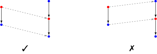
For any x∈Xx\in X and y∈Yy\in Y, if f(x)→𝕐yf(x)\to_{\mathbb{Y}}y, then there exists x′∈𝕏x^{\prime}\in\mathbb{X} such that x→𝕏x′x\to_{\mathbb{X}}x^{\prime} and f⁡(x′)=yf(x^{\prime})=y. (see Figure 11)

Notation 3.13.

The category of games and game morphisms is denoted by 𝐆𝐚𝐦𝐞\mathbf{Game}, and the canonical forgetful functor 𝕏=(X,→)↦X\mathbb{X}=(X,{\to})\mapsto X is denoted by U:𝐆𝐚𝐦𝐞→𝐒𝐞𝐭U\colon\mathbf{Game}\to\mathbf{Set}.

Summarizing the content of the previous and the current subsections, we arrive at the following so-called “theorem,” which is in effect little more than a systematic restatement of the definitions introduced so far.

Theorem 3.14 (Games as recursive coalgebras).

The category of games is equivalent55 5 In fact, they are isomorphic. to the category of recursive 𝒫fin\mathcal{P}_{\mathrm{fin}}-coalgebras.

𝐆𝐚𝐦𝐞≃𝐑𝐞𝐜𝐂𝐨𝐚𝐥𝐠𝒫fin\mathbf{Game}\simeq\mathbf{RecCoalg}_{\mathcal{P}_{\mathrm{fin}}}
Proof.

This follows from Proposition 3.10 and the argument above Definition 3.12. ∎

Some readers might find this “path-lifting” condition unnatural and hard to accept. On the one hand, some game theorists might think that it is a “category-theory-biased” condition with little connection to game theoretic phenomena. On the other hand, some category theorists might worry that the path-lifting property could break pleasant properties of the category of graphs. I believe these concerns will be resolved in the rest of the paper, but let us close this subsection with a brief explanation of why the “path-lifting property” is reasonable.

From a game theoretic perspective, the reason why we need the path-lifting property is simply because graph homomorphisms do not preserve game-theoretic data, such as the outcome and the Grundy number. For example, Figure 11 illustrates two graph morphisms: the left-hand one satisfies the path-lifting property and preserves the outcome, while the right-hand one does not. In fact, we will prove that all game morphisms preserve all “recursively defined” game data, such as the outcome and the Grundy number (Proposition 3.18 and Corollary 3.25).
Diagram
Figure 11. A game morphism (left side) and a graph morphism that does not satisfy the path-lifting property (right side) with PP-states and NN-states

From the categorical point of view, the category of games 𝐆𝐚𝐦𝐞\mathbf{Game} behaves surprisingly nice. Investigating the categorical properties of the category of games is not the main topic of this paper, but here I will list some facts.

Theorem 3.15 (Categorical properties of the category of games).

The category of games 𝐆𝐚𝐦𝐞\mathbf{Game} has the following properties:

  • •

    The category of games 𝐆𝐚𝐦𝐞\mathbf{Game} is locally finitely presentable. In particular, it has all small limits and colimits.

  • •

    The forgetful functor U:𝐆𝐚𝐦𝐞→𝐒𝐞𝐭U\colon\mathbf{Game}\to\mathbf{Set} is comonadic. In particular, it preserves, reflects, and strictly creates all small colimits.

  • •

    The category of games 𝐆𝐚𝐦𝐞\mathbf{Game} has a subobject classifier.

Proof.

The proofs are postponed until Appendix B. ∎

Remark 3.16 (Game is not just a graph with properties.).

In Definition 2.1, we defined the notion of games as if they were just graphs with some properties. However, that way of speaking is not accurate in the spirit of the categorical distinction between stuff, structure, and properties, since the canonical forgetful functor

𝐆𝐚𝐦𝐞→𝐆𝐫𝐚𝐩𝐡𝐬\mathbf{Game}\to\mathbf{Graphs}

is not fully faithful. (see [BS09, 2.4. Stuff, structure, and properties] for more explanation on the categorical distinction.) This fact is also mentioned in [Baš+24, Section 5]. In [Adá05], Adámek also points out that to regard 𝒫fin\mathcal{P}_{\mathrm{fin}}-coalgebras as graphs is “not a reasonable point of view” as follows:

[Adá05, Example 2.7.] Sometimes one also identifies QQ with a finitely branching directed graph […] However, this is often not a reasonable point of view because the coalgebra homomorphisms are much stronger than graph homomorphisms […]

Therefore, defining a game as a recursive coalgebra does not mean reducing it to graph theory. Rather, it extracts the structure — the “neighborhood function” θ\theta — from the underlying graph, and declares that this is the game-theoretic structure.

3.5. Game values as 𝒫fin\mathcal{P}_{\mathrm{fin}}-algebras

In this subsection, we explain how game values, such as outcome and the Grundy number, are understood in our categorical framework. First, we introduce the most naïve notion of the game value: the quantity preserved by all game morphisms.

Definition 3.17.

A game value is a cocone under the forgetful functor U:𝐆𝐚𝐦𝐞→𝐒𝐞𝐭U\colon\mathbf{Game}\to\mathbf{Set}. In other words, a game value 𝗏\mathsf{v} is a set AA equipped with a (proper class size) family of functions from all games

{𝗏𝕏:X→A}𝕏=(X,θ): game\{\mathsf{v}_{\mathbb{X}}\colon X\to A\}_{\mathbb{X}=(X,\theta)\text{: game}}

that is preserved by any game morphism f:𝕏→𝕐f\colon\mathbb{X}\to\mathbb{Y} in the sense that 𝗏𝕏=𝗏𝕐∘f\mathsf{v}_{\mathbb{X}}=\mathsf{v}_{\mathbb{Y}}\circ f.

𝕏; A; 𝕐; 𝗏𝕏; f; 𝗏𝕐

Thus, we obtain the following proposition as a special case of the abstract nonsense.

Proposition 3.18.

For any 𝒫fin\mathcal{P}_{\mathrm{fin}}-algebra 𝔸=(A,α)\mathbb{A}=(A,\alpha), the family of hylomorphisms

𝗁𝗒𝗅𝗈𝔸={𝗁𝗒𝗅𝗈𝔸,𝕏:X→A}𝕏=(X,θ): game\mathsf{hylo}_{\mathbb{A}}=\{\mathsf{hylo}_{\mathbb{A},\mathbb{X}}\colon X\to A\}_{\mathbb{X}=(X,\theta)\textrm{: game}}

is a game value.

Proof.

This is just a special case of the first half of Lemma 3.6. ∎

Let us see some examples of 𝒫fin\mathcal{P}_{\mathrm{fin}}-algebras and the induced game values. See Table 2 for the correspondence list.

Game value 𝒫fin\mathcal{P}_{\mathrm{fin}}-algebra
Outcome 𝖭𝖯=({N,P},𝗇𝗉)\mathsf{NP}=(\{N,P\},\mathsf{np})
Grundy number 𝖬𝖾𝗑=(ℕ,𝗆𝖾𝗑)\mathsf{Mex}=(\mathbb{N},\mathsf{mex})
Ended states 𝖤𝗆𝗉𝗍𝗒=({⊤,⊥},𝖾𝗆𝗉𝗍𝗒)\mathsf{Empty}=(\{\top,\bot\},\mathsf{empty})
Birthday 𝖷𝖾𝗆=(ℕ,𝗑𝖾𝗆)\mathsf{Xem}=(\mathbb{N},\mathsf{xem})
Misere outcome 𝖬𝖭𝖯=(ℕ,𝗆𝗇𝗉)\mathsf{MNP}=(\mathbb{N},\mathsf{mnp})
Remoteness (A,α)(A,\alpha) in Example 3.24
Table 2. Game values and the inducing 𝒫fin\mathcal{P}_{\mathrm{fin}}-algebras

First, let us observe that the outcome (Definition 2.2) and the Grundy number (Definition 2.14) are game values induced by 𝒫fin\mathcal{P}_{\mathrm{fin}}-algebras.

Example 3.19 (Outcome).

The outcome (Definition 2.2) 𝖮𝗎𝗍𝖼𝗈𝗆𝖾={𝖮𝗎𝗍𝖼𝗈𝗆𝖾𝕏:X→{N,P}}𝕏=(X,θ): game\mathsf{Outcome}=\{\mathsf{Outcome}_{\mathbb{X}}\colon X\to\{N,P\}\}_{\mathbb{X}=(X,\theta)\textrm{: game}} is induced by the 𝒫fin\mathcal{P}_{\mathrm{fin}}-algebra 𝖭𝖯=({N,P},𝗇𝗉)\mathsf{NP}=(\{N,P\},\mathsf{np}), where

𝗇𝗉:𝒫fin​({N,P})→{N,P}:S↦{P(P∉S)N(P∈S).\mathsf{np}\colon\mathcal{P}_{\mathrm{fin}}(\{N,P\})\to\{N,P\}\colon S\mapsto\begin{cases}P&(P\notin S)\\ N&(P\in S).\end{cases}

So we have

𝖮𝗎𝗍𝖼𝗈𝗆𝖾=𝗁𝗒𝗅𝗈𝖭𝖯.\mathsf{Outcome}=\mathsf{hylo}_{\mathsf{NP}}.
Example 3.20 (Grundy number).

The Grundy number 𝖦𝗋𝗎𝗇𝖽𝗒={𝖦𝗋𝗎𝗇𝖽𝗒𝕏:X→ℕ}\mathsf{Grundy}=\{\mathsf{Grundy}_{\mathbb{X}}\colon X\to\mathbb{N}\} (Definition 2.14) is induced by the 𝒫fin\mathcal{P}_{\mathrm{fin}}-algebra 𝖬𝖾𝗑=(ℕ,𝗆𝖾𝗑)\mathsf{Mex}=(\mathbb{N},\mathsf{mex}) (Definition 2.13).

𝖦𝗋𝗎𝗇𝖽𝗒=𝗁𝗒𝗅𝗈𝖬𝖾𝗑\mathsf{Grundy}=\mathsf{hylo}_{\mathsf{Mex}}

Other important game values in combinatorial game theory are also induced by 𝒫fin\mathcal{P}_{\mathrm{fin}}-algebras.

Example 3.21 (Ended states).

Let us start with an easy example. For each state x∈Xx\in X of a game 𝕏=(X,→)\mathbb{X}=(X,{\to}), we define 𝖤𝗇𝖽𝕏:X→{⊤,⊥}\mathsf{End}_{\mathbb{X}}\colon X\to\{\top,\bot\} by

𝖤𝗇𝖽𝕏(x)=⊤⇔the game ends at x⇔θ𝕏(x)=∅.\mathsf{End}_{\mathbb{X}}(x)=\top\iff\textrm{the game ends at $x$}\iff\theta_{\mathbb{X}}(x)=\emptyset.

This game value is induced by the 𝒫fin\mathcal{P}_{\mathrm{fin}}-algebra 𝖤𝗆𝗉𝗍𝗒=({⊤,⊥},𝖾𝗆𝗉𝗍𝗒)\mathsf{Empty}=(\{\top,\bot\},\mathsf{empty})

𝖾𝗆𝗉𝗍𝗒:𝒫fin​({⊤,⊥})→{⊤,⊥}:S↦{⊤(S=∅)⊥(S≠∅).\mathsf{empty}\colon\mathcal{P}_{\mathrm{fin}}(\{\top,\bot\})\to\{\top,\bot\}\colon S\mapsto\begin{cases}\top&(S=\emptyset)\\ \bot&(S\neq\emptyset).\end{cases}

So we obtain

𝖤𝗇𝖽=𝗁𝗒𝗅𝗈𝖤𝗆𝗉𝗍𝗒.\mathsf{End}=\mathsf{hylo}_{\mathsf{Empty}}.
Example 3.22 (Birthday).

For a game 𝕏=(X,→)\mathbb{X}=(X,{\to}) and a state x∈Xx\in X, its birthday66 6 The notion of birthday is usually defined for a set-theoretically constructed game, as an element of ℍ\mathbb{H}. Our version of the birthday of x∈Xx\in X coincides with the birthday of ξ𝕏​(x)∈ℍ\mathsf{\xi}_{\mathbb{X}}(x)\in\mathbb{H}., denoted by 𝖡𝗂𝗋𝗍𝗁𝖣𝖺𝗒𝕏​(x)\mathsf{BirthDay}_{\mathbb{X}}(x), is defined to be the length of the longest possible play from the state xx. This game value {𝖡𝗂𝗋𝗍𝗁𝖣𝖺𝗒𝕏:X→ℕ}\{\mathsf{BirthDay}_{\mathbb{X}}\colon X\to\mathbb{N}\} is induced by the 𝒫fin\mathcal{P}_{\mathrm{fin}}-algebra 𝖷𝖾𝗆=(ℕ,𝗑𝖾𝗆)\mathsf{Xem}=(\mathbb{N},\mathsf{xem})77 7 The notation 𝖷𝖾𝗆\mathsf{Xem} is not conventional. We adopt it because 𝖷𝖾𝗆\mathsf{Xem} is a kind of dual to 𝖬𝖾𝗑\mathsf{Mex}. See Appendix C for more details., where

𝗑𝖾𝗆:𝒫fin(ℕ)→ℕ:S↦min{n∈ℕ∣for any m∈S,m<n}.\mathsf{xem}\colon\mathcal{P}_{\mathrm{fin}}(\mathbb{N})\to\mathbb{N}\colon S\mapsto\min\{n\in\mathbb{N}\mid\textrm{for any }m\in S,m<n\}.

So we have

𝖡𝗂𝗋𝗍𝗁𝖣𝖺𝗒=𝗁𝗒𝗅𝗈𝖷𝖾𝗆.\mathsf{BirthDay}=\mathsf{hylo}_{\mathsf{Xem}}.
Example 3.23 (Misere outcome).

In combinatorial game theory, a misere game is a game where the player who takes the last move loses. In our framework, a misere game is understood by the same notion of a game, but a different notion of the outcome: the outcome should be modified so that the ending state is an NN-state. Defining a 𝒫fin\mathcal{P}_{\mathrm{fin}}-algebra 𝖬𝖭𝖯=({N,P},𝗆𝗇𝗉)\mathsf{MNP}=(\{N,P\},\mathsf{mnp}) by

𝗆𝗇𝗉:𝒫fin​({N,P})→{N,P}:S↦{P(S={N})N(S≠{N}),\mathsf{mnp}\colon\mathcal{P}_{\mathrm{fin}}(\{N,P\})\to\{N,P\}\colon S\mapsto\begin{cases}P&(S=\{N\})\\ N&(S\neq\{N\}),\end{cases}

the corresponding game evaluation is the misere outcome 𝖬𝖮𝗎𝗍𝖼𝗈𝗆𝖾=𝗁𝗒𝗅𝗈𝖬𝖭𝖯\mathsf{MOutcome}=\mathsf{hylo}_{\mathsf{MNP}}.

Example 3.24 (Remoteness [Smi66]).

If you do not just care about whether you win or lose, but also about how quickly you can win or how long you can postpone losing, then what you should look at is not the outcome but a more informative game value called the remoteness. The remoteness takes values in A={P2​k∣k∈ℕ}∪{N2​k+1∣k∈ℕ}A=\{P_{2k}\mid k\in\mathbb{N}\}\cup\{N_{2k+1}\mid k\in\mathbb{N}\}, where

  • •

    𝖱𝖾𝗆𝗈𝗍𝖾𝗇𝖾𝗌𝗌⁡(x)=P2​k\mathsf{Remoteness}(x)=P_{2k} means that, if you move to xx, then you can win in at most 2​k2k moves, and

  • •

    𝖱𝖾𝗆𝗈𝗍𝖾𝗇𝖾𝗌𝗌⁡(x)=N2​k+1\mathsf{Remoteness}(x)=N_{2k+1} means that, if you move to xx, you can avoid losing for at least 2​k+12k+1 moves.

This is a recuresively defined game value induced by the 𝒫fin\mathcal{P}_{\mathrm{fin}}-algebra structure

α⁡(S)≔{Nmin⁡{n∣Pn∈S}+1(if S contains some P)P𝗑𝖾𝗆​{n∣Nn∈S}(if S contains only N).\alpha(S)\coloneqq\begin{cases}N_{\min\{n\mid P_{n}\in S\}+1}&(\textrm{if $S$ contains some $P$})\\ P_{\mathsf{xem}\{n\mid N_{n}\in S\}}&(\textrm{if $S$ contains only $N$}).\end{cases}
Corollary 3.25.

Any game morphism preserves the outcome, the Grundy number, ended states, the birthday, the misere outcome, and the remoteness.

Proof.

These are just examples of Proposition 3.18, and hence examples of the stability of hylomorphisms (Lemma 3.6). ∎

Using the latter part of Lemma 3.6, we obtain the following statement:

Proposition 3.26.

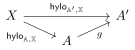
For any 𝒫fin\mathcal{P}_{\mathrm{fin}}-algebra homomorphism g:𝔸→𝔸′g\colon\mathbb{A}\to\mathbb{A}^{\prime} from 𝔸=(A,α)\mathbb{A}=(A,\alpha) to 𝔸′=(A′,α′)\mathbb{A}^{\prime}=(A^{\prime},\alpha^{\prime}), the game value 𝗁𝗒𝗅𝗈𝔸′\mathsf{hylo}_{\mathbb{A}^{\prime}} can be calculated via 𝗁𝗒𝗅𝗈𝔸\mathsf{hylo}_{\mathbb{A}}, i.e., we have 𝗁𝗒𝗅𝗈𝔸′,𝕏=g∘𝗁𝗒𝗅𝗈𝔸,𝕏\mathsf{hylo}_{\mathbb{A}^{\prime},\mathbb{X}}=g\circ\mathsf{hylo}_{\mathbb{A},\mathbb{X}}.

X; A′; A; 𝗁𝗒𝗅𝗈𝔸′,𝕏; 𝗁𝗒𝗅𝗈𝔸,𝕏; g
Proof.

This is just the latter half of Lemma 3.6. ∎

For example, the fact that 𝖮𝗎𝗍𝖼𝗈𝗆𝖾\mathsf{Outcome} is calculated by 𝖦𝗋𝗎𝗇𝖽𝗒\mathsf{Grundy} (Proposition 2.15) immediately follows from Proposition 3.26 and the fact that g:ℕ→{N,P}g\colon\mathbb{N}\to\{N,P\} defined by

g⁡(n)≔{N(n>0)P(n=0)g(n)\coloneqq\begin{cases}N&(n>0)\\ P&(n=0)\end{cases}

is a 𝒫fin\mathcal{P}_{\mathrm{fin}}-algebra homomorphism 𝖬𝖾𝗑→𝖭𝖯\mathsf{Mex}\to\mathsf{NP}. We can do similar arguments for the following 𝒫fin\mathcal{P}_{\mathrm{fin}}-algebra homomorphisms as well:

  • •

    𝖤𝗇𝖽\mathsf{End} is calculated by 𝖡𝗂𝗋𝗍𝗁𝖣𝖺𝗒\mathsf{BirthDay}.

  • •

    𝖤𝗇𝖽\mathsf{End} is calculated by 𝖱𝖾𝗆𝗈𝗍𝖾𝗇𝖾𝗌𝗌\mathsf{Remoteness}.

  • •

    𝖮𝗎𝗍𝖼𝗈𝗆𝖾\mathsf{Outcome} is calculated by 𝖱𝖾𝗆𝗈𝗍𝖾𝗇𝖾𝗌𝗌\mathsf{Remoteness}.

Remark 3.27 (Comparison with [Baš+24]).

As explained in Section 1, this subsection has a lot of intersection with [Baš+24]. Our Proposition 3.18 corresponds to their notion of valuations [Baš+24, Definition 4.11] and [Baš+24, Proposition 4.17]. Many examples of game values in this subsection also appear in [Baš+24, Section 4].

3.6. The terminal game consists of hereditarily finite sets

This subsection aims to describe the terminal game, which plays the central role in the next section (Section 4). First, we will describe it categorically (Diagram 4), and then we will write it down in a set-theoretic way (Proposition 3.31).

The calculation of the terminal recursive TT-coalgebra (== the terminal game, in our case) is a priori nontrivial. However, thanks to Proposition 3.7, it is reduced to the classical theorem of transfinite construction of an initial TT-algebra [Poh73, Adá74], which is known as Adamek’s fixed point theorem. (A concise explanation of the theorem, which suffices for our purpose, is found in [Jac16, Proposition 4.6.1 (1)].) The construction states that the initial algebra of 𝒫fin:𝐒𝐞𝐭→𝐒𝐞𝐭\mathcal{P}_{\mathrm{fin}}\colon\mathbf{Set}\to\mathbf{Set}, which also provides the terminal object in 𝐆𝐚𝐦𝐞≃𝐑𝐞𝐜𝐂𝐨𝐚𝐥𝐠𝒫fin\mathbf{Game}\simeq\mathbf{RecCoalg}_{\mathcal{P}_{\mathrm{fin}}} (Proposition 3.7), is given by the following colimit in 𝐒𝐞𝐭\mathbf{Set}

(4) ∅; 𝒫fin(∅); 𝒫fin(𝒫fin(∅)); 𝒫fin(𝒫fin(𝒫fin(∅))); ⋯The Terminal Game!

Here, we utilize the finite option condition in Definition 2.1 to ensure the assumption of Adamek’s fixed point theorem; the functor 𝒫fin:𝐒𝐞𝐭→𝐒𝐞𝐭\mathcal{P}_{\mathrm{fin}}\colon\mathbf{Set}\to\mathbf{Set} is finitary and hence preserves this colimit (cf. Remark 2.4).

Let us write down this colimit. (A canonical choice of) this colimit is known as the set of hereditarily finite sets in set theory. For its set-theoretic context and the terminology, see textbooks including [Kun13, section I.10].

Definition 3.28 (Hereditarily finite sets).

A hereditarily finite set is recursively defined as a finite set of hereditarily finite sets88 8 Rigorously speaking, a hereditarily finite set is a set that is ensured to be hereditarily finite by this recursive definition.. The set of all hereditarily finite sets is denoted by ℍ\mathbb{H}.

As this recursive definition might look confusing at first glance, let us give several examples.

Example 3.29.

The following sets are hereditarily finite sets:

  • •

    The empty set ∅\emptyset is trivially hereditarily finite since it has no element.

  • •

    Then, the set {∅}\{\emptyset\} is also hereditarily finite.

  • •

    By induction, every (von Neumann’s formulation of) natural number n={0,1,…​n−1}n=\{0,1,\dots n-1\} is hereditarily finite. In other words, we have

    ℕ={0=∅, 1={∅}, 2={∅,{∅}}, 3={∅,{∅},{∅,{∅}}},…}⊂ℍ.\mathbb{N}=\{0=\emptyset,\ 1=\{\emptyset\},\ 2=\{\emptyset,\{\emptyset\}\},\ 3=\{\emptyset,\{\emptyset\},\{\emptyset,\{\emptyset\}\}\},\;\dots\;\}\subset\mathbb{H}.
  • •

    The set {{∅}}\{\{\emptyset\}\} is a hereditarily finite set that is not a natural number.

  • •

    Informally speaking, hereditarily finite sets are sets described by a finite number of parentheses, like {{},{{{}}},{{}}}\{\{\},\{\{\{\}\}\},\{\{\}\}\}.

  • •

    While all hereditarily finite sets are finite, the converse does not hold. For example, while the set {ℝ}\{\mathbb{R}\} is a singleton, but it is not hereditarily finite.

Remark 3.30 (von Neumann hierarchy).

ℍ\mathbb{H} is often denoted by VωV_{\omega} in order to emphasize that it is the ω\omega-th of the von Neumann hierarchy.

By definition, 𝒫fin​(ℍ)\mathcal{P}_{\mathrm{fin}}(\mathbb{H}) is set-theoretically identical to ℍ\mathbb{H}. Therefore, ℍ\mathbb{H} admits

the canonical 𝒫fin\mathcal{P}_{\mathrm{fin}}-algebra structure   idℍ:ℍ→𝒫fin​(ℍ)​, and\displaystyle\mathrm{id}_{\mathbb{H}}:\mathbb{H}\to\mathcal{P}_{\mathrm{fin}}(\mathbb{H})\textrm{, and}
the canonical 𝒫fin\mathcal{P}_{\mathrm{fin}}-coalgebra structure   idℍ:𝒫fin​(ℍ)→ℍ.\displaystyle\mathrm{id}_{\mathbb{H}}:\mathcal{P}_{\mathrm{fin}}(\mathbb{H})\to\mathbb{H}.
Proposition 3.31 (Terminal object of 𝐆𝐚𝐦𝐞\mathbf{Game}).

The set ℍ\mathbb{H} is the initial 𝒫fin\mathcal{P}_{\mathrm{fin}}-algebra with the 𝒫fin\mathcal{P}_{\mathrm{fin}}-algebra structure idℍ:ℍ→𝒫fin​(ℍ)\mathrm{id}_{\mathbb{H}}:\mathbb{H}\to\mathcal{P}_{\mathrm{fin}}(\mathbb{H}). Therefore, ℍ\mathbb{H} is also the terminal object of 𝐆𝐚𝐦𝐞≃𝐑𝐞𝐜𝐂𝐨𝐚𝐥𝐠𝒫fin\mathbf{Game}\simeq\mathbf{RecCoalg}_{\mathcal{P}_{\mathrm{fin}}} with the 𝒫fin\mathcal{P}_{\mathrm{fin}}-coalgebra structure idℍ:𝒫fin​(ℍ)→ℍ\mathrm{id}_{\mathbb{H}}:\mathcal{P}_{\mathrm{fin}}(\mathbb{H})\to\mathbb{H}.

Proof.

The former part follows from Adamek’s fixed point theorem (see Diagram 4 and the discussion above). The latter follows from Proposition 3.7. ∎

By a mild abuse of notation, we will write ℍ\mathbb{H} for the set of hereditarily finite sets, the initial 𝒫fin\mathcal{P}_{\mathrm{fin}}-algebra, and the terminal recursive 𝒫fin\mathcal{P}_{\mathrm{fin}}-coalgebra.

It is worth writing down the relation →ℍ\to_{\mathbb{H}} of the terminal game ℍ\mathbb{H}.

Definition 3.32 (Terminal game).

The terminal game ℍ=(ℍ,→ℍ)\mathbb{H}=(\mathbb{H},\to_{\mathbb{H}}) is the game whose underlying set is the set of all hereditarily finite sets ℍ\mathbb{H} and whose relation →ℍ\to_{\mathbb{H}} is given by

x→ℍy⇔y∈x.x\to_{\mathbb{H}}y\iff y\in x.
Remark 3.33 (Ackerman’s interpretation and the binary exponent nim).

As we promised, the terminal game is isomorphic to the binary exponent nim in Example 2.6! Consider the following 𝒫fin\mathcal{P}_{\mathrm{fin}}-algebra structure on ℕ\mathbb{N}

𝖻𝗂𝗇:𝒫fin​(ℕ)→ℕ:S↦∑s∈S2s,\mathsf{bin}:\mathcal{P}_{\mathrm{fin}}(\mathbb{N})\to\mathbb{N}\colon S\mapsto\sum_{s\in S}2^{s},

which is just the binary expression and hence bijective. The unique 𝒫fin\mathcal{P}_{\mathrm{fin}}-algebra homomorphism 𝖠𝖼𝗄:(ℍ,idℍ)→(ℕ,𝖻𝗂𝗇)\mathsf{Ack}\colon(\mathbb{H},\mathrm{id}_{\mathbb{H}})\to(\mathbb{N},\mathsf{bin}) is called Ackerman’s interpretation [Ack37] and known to be bijective. Therefore, this 𝒫fin\mathcal{P}_{\mathrm{fin}}-algebra (ℕ,𝖻𝗂𝗇)(\mathbb{N},\mathsf{bin}) is isomorphic to the initial 𝒫fin\mathcal{P}_{\mathrm{fin}}-algebra (ℍ,idℍ)(\mathbb{H},\mathrm{id}_{\mathbb{H}}) and hence initial as well. Consequently, the inverse function 𝖻𝗂𝗇−1:ℕ→𝒫fin​(ℕ)\mathsf{bin}^{-1}\colon\mathbb{N}\to\mathcal{P}_{\mathrm{fin}}(\mathbb{N}), which coincides with the binary exponent nim, is also a terminal object in 𝐆𝐚𝐦𝐞≃𝐑𝐞𝐜𝐂𝐨𝐚𝐥𝐠𝒫fin\mathbf{Game}\simeq\mathbf{RecCoalg}_{\mathcal{P}_{\mathrm{fin}}}.

Notation 3.34.

For each game 𝕏\mathbb{X}, the unique game morphism to the terminal game ℍ\mathbb{H} is denoted by ξ𝕏:𝕏→ℍ\mathsf{\xi}_{\mathbb{X}}\colon\mathbb{X}\to\mathbb{H}.

Example 3.35.

For the 11-heap nim Nim1=(ℕ,θ)\mathrm{Nim}_{1}=(\mathbb{N},\theta), the game morphism ξNim1:ℕ→ℍ\mathsf{\xi}_{\mathrm{Nim}_{1}}\colon\mathbb{N}\to\mathbb{H} is nothing other than the von Neumann formulation of natural numbers. (cf. Example 3.11)

Lemma 3.36 (Characterization of game values).

For a (class-size) family of functions 𝗏={𝗏𝕏:X→B}𝕏=(X,θ): game\mathsf{v}=\{\mathsf{v}_{\mathbb{X}}\colon X\to B\}_{\mathbb{X}=(X,\theta)\textrm{: game}}, the following conditions are equivalent.

  1. (1)

    The family 𝗏\mathsf{v} is a game value (Definition 3.17), i.e., any game morphism preserves 𝗏\mathsf{v}.

  2. (2)

    The equality 𝗏𝕏=𝗏ℍ∘ξ𝕏\mathsf{v}_{\mathbb{X}}=\mathsf{v}_{\mathbb{H}}\circ\mathsf{\xi}_{\mathbb{X}} holds for any game 𝕏\mathbb{X}.

  3. (3)

    There exists a 𝒫fin\mathcal{P}_{\mathrm{fin}}-algebra 𝔸=(A,α)\mathbb{A}=(A,\alpha) and a function g:A→Bg\colon A\to B such that 𝗏𝕏=g∘𝗁𝗒𝗅𝗈𝔸,𝕏\mathsf{v}_{\mathbb{X}}=g\circ\mathsf{hylo}_{\mathbb{A},\mathbb{X}} for any game 𝕏\mathbb{X}.

Proof.

The implication (1)⟹(2)(1)\implies(2) follows since ξ𝕏:𝕏→ℍ\mathsf{\xi}_{\mathbb{X}}\colon\mathbb{X}\to\mathbb{H} is a game morphism. The implication (2)⟹(3)(2)\implies(3) follows since we can take the initial 𝒫fin\mathcal{P}_{\mathrm{fin}}-algebra ℍ\mathbb{H} as 𝔸\mathbb{A}, and 𝗏ℍ\mathsf{v}_{\mathbb{H}} as gg using the terminal game ℍ\mathbb{H} (cf. Proposition 3.31). The last implication (3)⟹(1)(3)\implies(1) follows from Proposition 3.18. ∎

Remark 3.37 (ℍ\mathbb{H} as colimit, and a game with a starting state.).

For category theorists, Lemma 3.36 is an immediate corollary of an almost trivial fact that ℍ\mathbb{H} is the colimit of the forgetful functor U:𝐆𝐚𝐦𝐞→𝐒𝐞𝐭U\colon\mathbf{Game}\to\mathbf{Set}, and the morphisms {ξ𝕏:X→ℍ}𝕏=(X,θ): game\{\mathsf{\xi}_{\mathbb{X}}\colon X\to\mathbb{H}\}_{\mathbb{X}=(X,\theta)\textrm{: game}} is the colimit cocone of this large colimit. Since the category 𝐆𝐚𝐦𝐞\mathbf{Game} has the terminal object ℍ\mathbb{H}, the colimit of this diagram is just the image of the terminal object ℍ\mathbb{H}. As game values are defined as cocones of UU (Definition 3.17), one can say that ℍ\mathbb{H} is the “universal game value” (but in a bit boring way).

This phenomenon is loosely related to the relationships between different definitions of games. In some context, an impartial game is defined as an element of ℍ\mathbb{H}. From our point of view, each element x∈Xx\in X defines a “game” ξ𝕏​(x)∈ℍ\mathsf{\xi}_{\mathbb{X}}(x)\in\mathbb{H} in that sense. In slightly different words, if we consider games 𝕏\mathbb{X} equipped with a “starting state” x∈𝕏x\in\mathbb{X}, we can define the category of pointed games 𝐆𝐚𝐦𝐞∗\mathbf{Game}_{*}, whose connected components are in one-to-one correspondence with hereditarily finite sets:

π0(𝐆𝐚𝐦𝐞∗)=π0(∫U)=colim(U:𝐆𝐚𝐦𝐞→𝐒𝐞𝐭)=ℍ.\pi_{0}\left(\mathbf{Game}_{*}\right)=\pi_{0}\left(\int U\right)=\colim\left(U\colon\mathbf{Game}\to\mathbf{Set}\right)=\mathbb{H}.
Remark 3.38.

As the condition (3) in Lemma 3.36 infers, some game values are not induced by 𝒫fin\mathcal{P}_{\mathrm{fin}}-algebras. In fact, while the number of 𝒫fin\mathcal{P}_{\mathrm{fin}}-algebra structures on the 22-element set {⊤,⊥}\{\top,\bot\} is #​{⊤,⊥}𝒫fin​({⊤,⊥})=16\#\{\top,\bot\}^{\mathcal{P}_{\mathrm{fin}}(\{\top,\bot\})}=16, there are exactly #​{⊤,⊥}ℍ=2ℵ0\#\{\top,\bot\}^{\mathbb{H}}=2^{\aleph_{0}} distinct game values on it due to Lemma 3.36.

4. Application: Nim-sum type theorem schema and the Bouton monoids

As an example of usages of our framework, this section provides a theorem schema that generalizes the nim-sum rule (Theorem 2.17). We firstly define the notion of a Bouton monoid (Definition 4.6), and then prove that it always exists (Theorem 4.8).

∗; 𝗏; ℬ∗,𝗏; 𝖻
Figure 12. How theorem schema works
+; 𝖮𝗎𝗍𝖼𝗈𝗆𝖾; (ℕ,⊕); 𝖦𝗋𝗎𝗇𝖽𝗒
Figure 13. The nim-sum as an example of the theorem schema

4.1. Decomposing games with monoidal structures

The goal of this subsection is to find a systematic way to decompose a complex game into simpler games. An established categorical tool to decompose objects is a monoidal structure on a category. For those who are not familiar with this notion, a standard reference is [Mac98].

In this subsection, we will observe several monoidal structures on the category 𝐆𝐚𝐦𝐞\mathbf{Game}.

Remark 4.1.

In this section, we also consider non-unital monoidal category, which does not require the unit object. Everything in this section works by replacing monoidal by non-unital monoidal, and monoid by semigroup. If the reader is not familiar with non-unital monoidal structure, one can restrict arguments to the unital cases, while considering remoteness will require non-unital one (Example 4.16).

Hisorically, the Conway addition is regarded as the canonical choice of monoidal structure on categories of games (for example, [Joy77]). It also provides a monoidal structure on our category.

Proposition 4.2.

The Conway addition is a symmetric monoidal closed structure on 𝐆𝐚𝐦𝐞\mathbf{Game} with the monoidal unit 1=({∗},→1=∅)1=(\{*\},\to_{1}=\emptyset).

Proof.

Being symmetric monoidal is easily proven. The closedness, which we will not use in this section, is proven in Corollary B.11. ∎

Let us see some other examples.

Example 4.3 (Selective sum [Smi66]).

For a finite number of games 𝕏1,…,𝕏n\mathbb{X}_{1},\dots,\mathbb{X}_{n} with n≥0n\geq 0, their selective sum 𝕏1∨⋯∨𝕏n\mathbb{X}_{1}\lor\dots\lor\mathbb{X}_{n} is the game in which each player selects at least one games out of the nn games and makes one move for each selected game. More foramlly spealing, the selective sum 𝕏∨𝕐\mathbb{X}\lor\mathbb{Y} of two games 𝕏=(X,→𝕏),𝕐=(Y,→𝕐)\mathbb{X}=(X,\to_{\mathbb{X}}),\mathbb{Y}=(Y,\to_{\mathbb{Y}}) is defined as follows:

  • •

    Its underlying set is X×YX\times Y.

  • •

    (x,y)→𝕏∨𝕐(x′,y′)(x,y)\to_{\mathbb{X}\lor\mathbb{Y}}(x^{\prime},y^{\prime}) is defined by

    (x,y)→𝕏∨𝕐(x′,y′)⇔(x→𝕏x′∧y=y′)∨(x→𝕏x′∧y→𝕐y′)∨(x=x′∧y→𝕐y′)(x,y)\to_{\mathbb{X}\lor\mathbb{Y}}(x^{\prime},y^{\prime})\iff(x\to_{\mathbb{X}}x^{\prime}\land y=y^{\prime})\lor(x\to_{\mathbb{X}}x^{\prime}\land y\to_{\mathbb{Y}}y^{\prime})\lor(x=x^{\prime}\land y\to_{\mathbb{Y}}y^{\prime})

The selective sum defines a (unital, symmetric, and closed) monoidal structure on 𝐆𝐚𝐦𝐞\mathbf{Game} with the monoidal unit 1=({∗},→1=∅)1=(\{*\},\to_{1}=\emptyset).

Example 4.4 (Conjunctive sum [Smi66]).

For a finite and positive number of games 𝕏1,…,𝕏n\mathbb{X}_{1},\dots,\mathbb{X}_{n} with n>0n>0, their conjunctive sum 𝕏1∧⋯∧𝕏n\mathbb{X}_{1}\land\dots\land\mathbb{X}_{n} is the game in which each player makes a move for all of the nn games. More foramlly spealing, the conjunctive sum 𝕏∧𝕐\mathbb{X}\land\mathbb{Y} of two games 𝕏=(X,→𝕏),𝕐=(Y,→𝕐)\mathbb{X}=(X,\to_{\mathbb{X}}),\mathbb{Y}=(Y,\to_{\mathbb{Y}}) is defined as follows:

  • •

    Its underlying set is X×YX\times Y.

  • •

    (x,y)→𝕏∧𝕐(x′,y′)(x,y)\to_{\mathbb{X}\land\mathbb{Y}}(x^{\prime},y^{\prime}) is defined by

    (x,y)→𝕏∨𝕐(x′,y′)⇔(x→𝕏x′∧y→𝕐y′)(x,y)\to_{\mathbb{X}\lor\mathbb{Y}}(x^{\prime},y^{\prime})\iff(x\to_{\mathbb{X}}x^{\prime}\land y\to_{\mathbb{Y}}y^{\prime})

The conjuctive sum defines a non-unital99 9 The conjunctive sum defines a monoidal structure on 𝐂𝐨𝐚𝐥𝐠𝒫fin\mathbf{Coalg}_{\mathcal{P}_{\mathrm{fin}}} with a monoidal unit (Figure 5), which fails to be a game. (but symmetric and closed) monoidal structure on 𝐆𝐚𝐦𝐞\mathbf{Game}.

4.2. Synthesizing game values with Bouton monoids

4.2.1. Bouton monoid

In the story of the Bouton theorem (Section 2), the abelian group of the nim-sum (ℕ,⊕)(\mathbb{N},\oplus) (Definition 2.16) and the notion of Grundy number 𝖦𝗋𝗎𝗇𝖽𝗒={𝖦𝗋𝗎𝗇𝖽𝗒𝕏:X→ℕ}𝕏=(X,θ): game\mathsf{Grundy}=\{\mathsf{Grundy}_{\mathbb{X}}\colon X\to\mathbb{N}\}_{\mathbb{X}=(X,\theta)\textrm{: game}} plays a central role. More concretely, there are two characterizing properties of them:

(1) Informative (Proposition 2.15):

For any game 𝕏\mathbb{X} and any element x∈Xx\in X, the Grundy number is more informative than the outcome in the sense that

𝖮𝗎𝗍𝖼𝗈𝗆𝖾𝕏​(x)=P⇔𝖦𝗋𝗎𝗇𝖽𝗒𝕏​(x)=0.\mathsf{Outcome}_{\mathbb{X}}(x)=P\iff\mathsf{Grundy}_{\mathbb{X}}(x)=0.
(2) Decomposable (Theorem 2.17):

For any games 𝕏=(X,θ𝕏),𝕐=(Y,θ𝕐)\mathbb{X}=(X,\theta_{\mathbb{X}}),\mathbb{Y}=(Y,\theta_{\mathbb{Y}}) and any states x∈X,y∈Yx\in X,y\in Y, the Grundy number of the sum state (x,y)∈𝕏+𝕐(x,y)\in\mathbb{X}+\mathbb{Y} is decomposable in the sense that

𝖦𝗋𝗎𝗇𝖽𝗒𝕏+𝕐​(x,y)=𝖦𝗋𝗎𝗇𝖽𝗒𝕏​(x)⊕𝖦𝗋𝗎𝗇𝖽𝗒𝕐​(y).\mathsf{Grundy}_{\mathbb{X}+\mathbb{Y}}(x,y)=\mathsf{Grundy}_{\mathbb{X}}(x)\oplus\mathsf{Grundy}_{\mathbb{Y}}(y).

We will define the notion of a Bouton monoid as the minimum monoid that satisfies the two conditions above. The existence will be proven later (Theorem 4.8).

In the follwoing definition, we will use the notion of lax monoidal functors. For those who are not familiar with that notion, one can just consider monoidal structure ∗\ast on 𝐆𝐚𝐦𝐞\mathbf{Game} that makes UU strictly monoidal, i.e., U​𝕏×U​𝕐=U⁡(𝕏∗𝕐)U\mathbb{X}\times U\mathbb{Y}=U(\mathbb{X}\ast\mathbb{Y}). In fact, all the three monoidal structures in Section 4.1 make U:𝐆𝐚𝐦𝐞→𝐒𝐞𝐭U\colon\mathbf{Game}\to\mathbf{Set} strict monoidal.

Notation 4.5 (Notations around lax monoidal functors).

If one consider a monoidal structure ∗\ast on the category 𝐆𝐚𝐦𝐞\mathbf{Game} that makes U:𝐆𝐚𝐦𝐞→𝐒𝐞𝐭U\colon\mathbf{Game}\to\mathbf{Set} lax monoidal1010 10 Rigorously speaking, as the comparison map is a part of the lax monoidal functor, saying that “UU is lax monoidal” is somewhat misleading. Similarly, to be rigorous, we need to specify the associativity and the unitality maps of the monoidal structure. However, we intentionally hide these data by a conventional abuse of notation, partially because of Remark 4.1. (with respect to the cartesian monoidal structure on 𝐒𝐞𝐭\mathbf{Set}), we will write

μ𝕏,𝕐:U​𝕏×U​𝕐→U⁡(𝕏∗𝕐)\mu_{\mathbb{X},\mathbb{Y}}\colon U\mathbb{X}\times U\mathbb{Y}\to U(\mathbb{X}\ast\mathbb{Y})

for the chosen comparison map. Furthermore, for a pair of states (x,y)∈U​𝕏×U​𝕐(x,y)\in U\mathbb{X}\times U\mathbb{Y}, we will write (x,y)∈U⁡(𝕏∗𝕐)(x,y)\in U(\mathbb{X}\ast\mathbb{Y}) for the state μ𝕏,𝕐​(x,y)\mu_{\mathbb{X},\mathbb{Y}}(x,y). Notice that it is compatible with the notations in the previous sections, for example, in Theorem 2.17.

Now we are ready to state the definition of the Bouton monoid. To aid in understanding the definition, Table 3 shows the correspondence between the general case and the specific case of the nim-sum.

Definition 4.6.

Let ∗\ast be a monoidal structure on 𝐆𝐚𝐦𝐞\mathbf{Game} such that the forgetful functor U:𝐆𝐚𝐦𝐞→𝐒𝐞𝐭U\colon\mathbf{Game}\to\mathbf{Set} is lax monoidal, and let 𝗏={𝗏𝕏:X→A}𝕏=(X,θ): game\mathsf{v}=\{\mathsf{v}_{\mathbb{X}}\colon X\to A\}_{\mathbb{X}=(X,\theta)\textrm{: game}} be a game value. The Bouton monoid of ∗\ast and 𝗏\mathsf{v} is

  • •

    a game value 𝖻={𝖻𝕏:X→ℬ}\mathsf{b}=\{\mathsf{b}_{\mathbb{X}}\colon X\to\mathcal{B}\} equipped with

  • •

    a function a:ℬ→Aa\colon\mathcal{B}\to A and

  • •

    a monoid structure ⊛:ℬ×ℬ→ℬ\circledast\colon\mathcal{B}\times\mathcal{B}\to\mathcal{B}

that satisfies the following three conditions.

(1) Informative:

For any game 𝕏\mathbb{X}, we have

𝗏𝕏=a∘𝖻𝕏.\mathsf{v}_{\mathbb{X}}=a\circ\mathsf{b}_{\mathbb{X}}.
(2) Decomposable:

For any games 𝕏=(X,θ𝕏),𝕐=(Y,θ𝕐)\mathbb{X}=(X,\theta_{\mathbb{X}}),\mathbb{Y}=(Y,\theta_{\mathbb{Y}}) and any states x∈X,y∈Yx\in X,y\in Y, we have

𝖻𝕏∗𝕐​(x,y)=𝖻𝕏​(x)⊛𝖻𝕐​(y).\mathsf{b}_{\mathbb{X}\ast\mathbb{Y}}(x,y)=\mathsf{b}_{\mathbb{X}}(x)\circledast\mathsf{b}_{\mathbb{Y}}(y).
(3) Minimum:

It is minimum among such data. More concretely, for any data of the same type (𝖻′={𝖻𝕏′:X→ℬ′},a′:ℬ′→A,⊛′:ℬ′×ℬ′→ℬ′)(\mathsf{b}^{\prime}=\{\mathsf{b}^{\prime}_{\mathbb{X}}\colon X\to\mathcal{B}^{\prime}\},a^{\prime}\colon\mathcal{B}^{\prime}\to A,\circledast^{\prime}\colon\mathcal{B}^{\prime}\times\mathcal{B}^{\prime}\to\mathcal{B}^{\prime}) satisfying (the appropriate substitutes of) the above two conditions, there exsits a surjective monoid homomorphism q:∙↠ℬq\colon\bullet\twoheadrightarrow\mathcal{B} from a submonoid ∙⊂ℬ′\bullet\subset\mathcal{B}^{\prime} such that the following diagram

∙; ℬ′; X; A; ℬ; ⊂; q; a′; 𝖻𝕏′; 𝖻𝕏; a

commutes for any game 𝕏=(X,θ)\mathbb{X}=(X,\theta).

General case Nim-sum case
Monoidal structure ∗\ast Conway addition ++
(Target) game value 𝗏\mathsf{v} 𝖮𝗎𝗍𝖼𝗈𝗆𝖾\mathsf{Outcome}
μ𝕏,𝕐\mu_{\mathbb{X},\mathbb{Y}} idX×Y\mathrm{id}_{X\times Y}
𝖻𝕏\mathsf{b}_{\mathbb{X}} 𝖦𝗋𝗎𝗇𝖽𝗒𝕏\mathsf{Grundy}_{\mathbb{X}}
ℬ\mathcal{B} ℕ\mathbb{N}
⊛\circledast Nim-sum ⊕\oplus
a:ℬ→Aa\colon\mathcal{B}\to A ℕ→{N,P}:0↦P\mathbb{N}\to\{N,P\}\colon 0\mapsto P
𝗏𝕏=a∘𝖻𝕏\mathsf{v}_{\mathbb{X}}=a\circ\mathsf{b}_{\mathbb{X}} Proposition 2.15
𝖻𝕏∗𝕐​(x,y)=𝖻𝕏​(x)⊛𝖻𝕐​(y)\mathsf{b}_{\mathbb{X}\ast\mathbb{Y}}(x,y)=\mathsf{b}_{\mathbb{X}}(x)\circledast\mathsf{b}_{\mathbb{Y}}(y) Theorem 2.17
Table 3. The correspondence table between the general cases and the nim-sum case
Remark 4.7 (Is this minimality condition weird?).

Some readers may be unfamiliar with this kind of minimality condition. But actually it is very common especially in the automata theory. For example, the minimality of automata and syntactic monoids (Example A.3) are stated in this form. See textbooks including [Pin22], and see also [CP20] for an elegant categorical framework. This minimality condition says that the Bouton monoid ℬ\mathcal{B} is a subquotient of any others, which informally means that ℬ\mathcal{B} has neither redundant elements (== no proper submonoids) nor redundunt fineness (== no proper quotient monoids).

The goal of this subsection is to prove the existence of the Bouton monoid.

Theorem 4.8 (Existence of Bouton monoid).

For any monoidal structure ∗\ast on 𝐆𝐚𝐦𝐞\mathbf{Game} such that the forgetful functor U:𝐆𝐚𝐦𝐞→𝐒𝐞𝐭U\colon\mathbf{Game}\to\mathbf{Set} is lax monoidal, and any game value 𝗏={𝗏𝕏:X→A}𝕏=(X,θ): game\mathsf{v}=\{\mathsf{v}_{\mathbb{X}}\colon X\to A\}_{\mathbb{X}=(X,\theta)\textrm{: game}}, the Bouton monoid exists.

4.2.2. Step 1: Miniature monoid

We start with constructing an approximation of the Bouton monoid only by the information of the monoidal structure ∗\ast forgetting the terget game value 𝗏\mathsf{v}. We will call the approximation by a temporary name: the miniture monoid of the monoidal structure ∗\ast.

The following trivial proposition is usually very boring due to the triviality of the terminal object. But it is worth considering in a category of coalgebras, in which a terminal object tends to be non-trivial.

Lemma 4.9.

For any monoidal category with a terminal object 11, the object 11 has a unique monoid structure with respect to the monoidal structure.

Proof.

In a monoidal category (𝒞,I,⊗)(\mathcal{C},I,\otimes) with a terminal object 11, the multiplication map m:1⊗1→1m\colon 1\otimes 1\to 1 (and the unit map e:I→1e\colon I\to 1 if you consider a unital structure) is uniquely determined since 11 is terminal. All required commutativities are trivial since 11 is the terminal object. ∎

In our case of the category of games 𝐆𝐚𝐦𝐞\mathbf{Game}, the unique game morphism ξℍ∗ℍ:ℍ∗ℍ→ℍ\mathsf{\xi}_{\mathbb{H}\ast\mathbb{H}}\colon\mathbb{H}\ast\mathbb{H}\to\mathbb{H} provides the unique ∗\ast-monoid structure on the terminal game ℍ\mathbb{H}. Then, we can convert the ∗\ast-monoid (ℍ,ξℍ∗ℍ:ℍ∗ℍ→ℍ)(\mathbb{H},\mathsf{\xi}_{\mathbb{H}\ast\mathbb{H}}\colon\mathbb{H}\ast\mathbb{H}\to\mathbb{H}) to a usual monoid by the following well-known fact.

Fact 4.10.

Any lax monoidal functor F:(𝒞,I𝒞,⊗𝒞)→(𝒟,I𝒟,⊗𝒟)F\colon(\mathcal{C},I_{\mathcal{C}},\otimes_{\mathcal{C}})\to(\mathcal{D},I_{\mathcal{D}},\otimes_{\mathcal{D}}) sends a monoid object in 𝒞\mathcal{C} to a monoid object in 𝒟\mathcal{D}.

By the assumption that U:𝐆𝐚𝐦𝐞→𝐒𝐞𝐭U\colon\mathbf{Game}\to\mathbf{Set} is lax monoidal, we obtain the induced monoid whose multiplacation function is given by

U​ℍ×U​ℍ→μℍ,ℍU⁡(ℍ∗ℍ)→U⁡(ξℍ∗ℍ)U​ℍ,U\mathbb{H}\times U\mathbb{H}\xrightarrow{\mu_{\mathbb{H},\mathbb{H}}}U(\mathbb{H}\ast\mathbb{H})\xrightarrow{U(\mathsf{\xi}_{\mathbb{H}\ast\mathbb{H}})}U\mathbb{H},

where μ𝕏,𝕐:U⁡(𝕏)×U⁡(𝕐)→U⁡(𝕏∗𝕐)\mu_{\mathbb{X},\mathbb{Y}}\colon U(\mathbb{X})\times U(\mathbb{Y})\to U(\mathbb{X}\ast\mathbb{Y}) denotes the comparison map of the lax monoidal functor UU. We will call this monoid structure on the set ℍ\mathbb{H} the miniature monoid of the monoidal structure ∗\ast, and write ∗ℍ:ℍ×ℍ→ℍ{\ast_{\mathbb{H}}}\colon\mathbb{H}\times\mathbb{H}\to\mathbb{H} for the multiplication function.

Example 4.11 (Miniture monoids for some monoidal structures).

For the Conway addition ++, the miniature monoid structure +ℍ+_{\mathbb{H}} on ℍ\mathbb{H} is given by

A+ℍB={a+ℍB∣a∈A}∪{A+ℍb∣b∈B}.A+_{\mathbb{H}}B=\{a+_{\mathbb{H}}B\mid a\in A\}\cup\{A+_{\mathbb{H}}b\mid b\in B\}.

In usual context like [Sie13], this is just called the Conway addition. Similarly, the miniature monoid structure of ∨\lor (Example 4.3) and ∧\land (Example 4.4) are given by

A∨ℍB\displaystyle A\lor_{\mathbb{H}}B ={a∨ℍB∣a∈A}∪{a∨ℍb∣a∈A,b∈B}∪{A∨ℍb∣b∈B} and\displaystyle=\{a\lor_{\mathbb{H}}B\mid a\in A\}\cup\{a\lor_{\mathbb{H}}b\mid a\in A,b\in B\}\cup\{A\lor_{\mathbb{H}}b\mid b\in B\}\text{ and}
A∧ℍB\displaystyle A\land_{\mathbb{H}}B ={a∧ℍb∣a∈A,b∈B}.\displaystyle=\{a\land_{\mathbb{H}}b\mid a\in A,b\in B\}.
Lemma 4.12 (Miniature monoid reflects the ambient monoidal structure).

For any pair of games 𝕏=(X,→𝕏)\mathbb{X}=(X,\to_{\mathbb{X}}) and 𝕐=(Y,→𝕐)\mathbb{Y}=(Y,\to_{\mathbb{Y}}), we have the following equation in the miniature monoid:

ξ𝕏∗𝕐​(x,y)=ξ𝕏​(x)∗ℍξ𝕐​(y).\mathsf{\xi}_{\mathbb{X}\ast\mathbb{Y}}(x,y)=\mathsf{\xi}_{\mathbb{X}}(x)\ast_{\mathbb{H}}\mathsf{\xi}_{\mathbb{Y}}(y).
Proof.

Since ℍ\mathbb{H} is the terminal game, we have the following commutative diagram in 𝐆𝐚𝐦𝐞\mathbf{Game}:

(5) 𝕏∗𝕐,; ℍ∗ℍ; ℍ.; ξ𝕏∗𝕐; ξ𝕏∗ξ𝕐; ξℍ∗ℍ

By sending this diagram by UU and utilizing the naturality of μ\mu, we have the following commutative diagram in 𝐒𝐞𝐭\mathbf{Set}:

X×Y=U𝕏×U𝕐; U⁡(𝕏∗𝕐),; ℍ×ℍ=Uℍ×Uℍ; U⁡(ℍ∗ℍ); U⁡(ℍ)=ℍ.; Uξ𝕏×Uξ𝕐; μ𝕏,𝕐; U⁡(ξ𝕏∗𝕐); U⁡(ξ𝕏∗ξ𝕐); μℍ,ℍ; ∗ℍ; U⁡(ξℍ∗ℍ)

This completes the proof. ∎

4.2.3. Step 2: Minimum monoid factorization

The miniture monoid (ℍ,∗ℍ)(\mathbb{H},\ast_{\mathbb{H}}) depends only on the monoidal structure ∗\ast, and is independent of the target game value 𝗏\mathsf{v}. So we want to minimize ℍ\mathbb{H} keeping the ability to calculate the target game value 𝗏\mathsf{v}. We introduce a very simple gadget for minimizing a monoid. See Appendix A for related contexts, examples, and the proof of the existence.

Definition 4.13 (Minimum monoid factorization).

For a monoid MM and a function f:M→Af\colon M\to A to a set AA, the minimum monoid factorization of f:M→Af\colon M\to A is a monoid MfM_{f} equipped with a factorization of the function ff into a monoid homomorphism qf:M→Mfq_{f}\colon M\to M_{f} followed by a function af:Mf→Aa_{f}\colon M_{f}\to A

M; Mf; A; f; qf; af

that satisfies the following minimality condition.

Minimum:

For any monoid Mf′M^{\prime}_{f} equipped with a factorization f=M→qf′Mf′→af′Af=M\xrightarrow{q^{\prime}_{f}}M^{\prime}_{f}\xrightarrow{a^{\prime}_{f}}A into a monoid homomorphism qf′:M→Mf′q^{\prime}_{f}\colon M\to M^{\prime}_{f} followed by a function af′:Mf′→Aa^{\prime}_{f}\colon M^{\prime}_{f}\to A, there exsits a surjective monoid homomorphism q:∙↠Mfq\colon\bullet\twoheadrightarrow M_{f} from a submonoid ∙⊂Mf′\bullet\subset M^{\prime}_{f} such that the following diagram commutes.
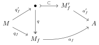
∙; Mf′; M; A; Mf; ⊂; q; af′; qf′; qf; af

One can check that the minimum monoid factorization always uniquely exists (up to canonical isomorphisms. See Proposition A.1 for a detailed proof and a construction. If one considers a non-unital monoidal structure (Remark 4.1), one can use the semigroup version in Remark A.4.

Let us return to the context of the Bouton monoid. Since ℍ\mathbb{H} has the miniture monoid structure (Section 4.2.2), we can consider the minimum monoid factorization of the function 𝗏ℍ:ℍ→A\mathsf{v}_{\mathbb{H}}\colon\mathbb{H}\to A. Let ℍ→q𝗏ℍℬ→a𝗏ℍA\mathbb{H}\xrightarrow{q_{\mathsf{v}_{\mathbb{H}}}}\mathcal{B}\xrightarrow{a_{\mathsf{v}_{\mathbb{H}}}}A be the minimum monoid factorization of the function 𝗏ℍ:ℍ→A\mathsf{v}_{\mathbb{H}}\colon\mathbb{H}\to A with respect to the miniature monoid structure ∗ℍ:ℍ×ℍ→ℍ\ast_{\mathbb{H}}\colon\mathbb{H}\times\mathbb{H}\to\mathbb{H}. Let ⊛:ℬ×ℬ→ℬ\circledast\colon\mathcal{B}\times\mathcal{B}\to\mathcal{B} denote the induced monoid structure on ℬ\mathcal{B}. For any game 𝕏=(X,θ)\mathbb{X}=(X,\theta), due to Lemma 3.36, we obtain the following decomposition of the function 𝗏𝕏:X→A\mathsf{v}_{\mathbb{X}}\colon X\to A.

X; ℍ; ℬ; A; ξ𝕏; 𝗏𝕏; q𝗏ℍ; 𝗏ℍ; a𝗏ℍ

We define 𝖻𝕏:X→ℬ\mathsf{b}_{\mathbb{X}}\colon X\to\mathcal{B} by 𝖻𝕏≔q𝗏ℍ∘ξ𝕏\mathsf{b}_{\mathbb{X}}\coloneqq q_{\mathsf{v}_{\mathbb{H}}}\circ\mathsf{\xi}_{\mathbb{X}}.

X; ℍ; ℬ; A.; ξ𝕏; 𝗏𝕏; 𝖻𝕏; q𝗏ℍ; 𝗏ℍ; a𝗏ℍ

The family of functions 𝖻={𝖻𝕏:X→ℬ}𝕏=(X,θ): game\mathsf{b}=\{\mathsf{b}_{\mathbb{X}}\colon X\to\mathcal{B}\}_{\mathbb{X}=(X,\theta)\textrm{: game}} is a game value, also due to Lemma 3.36 since it factors through ξ={ξ𝕏:X→ℍ}𝕏=(X,θ): game\mathsf{\xi}=\{\mathsf{\xi}_{\mathbb{X}}\colon X\to\mathbb{H}\}_{\mathbb{X}=(X,\theta)\textrm{: game}}.

We will prove that the triple of the game value 𝖻={𝖻𝕏:X→ℬ}𝕏=(X,θ): game\mathsf{b}=\{\mathsf{b}_{\mathbb{X}}\colon X\to\mathcal{B}\}_{\mathbb{X}=(X,\theta)\textrm{: game}}, the function a𝗏ℍ:ℬ→Aa_{\mathsf{v}_{\mathbb{H}}}\colon\mathcal{B}\to A, and the monoid structure ⊛:ℬ×ℬ→ℬ\circledast\colon\mathcal{B}\times\mathcal{B}\to\mathcal{B}, all defined just above, provides the Bouton monoid for ∗\ast and 𝗏\mathsf{v}. Regarding the first condition “(1) Informative”, the required equation 𝗏𝕏=a𝗏ℍ∘𝖻𝕏\mathsf{v}_{\mathbb{X}}=a_{\mathsf{v}_{\mathbb{H}}}\circ\mathsf{b}_{\mathbb{X}} obviously holds by definition. Regarding the second condition “(2) Decomposable”, we have

𝖻𝕏∗𝕐​(x,y)=q𝗏ℍ​(ξ𝕏∗𝕐​(x,y))=q𝗏ℍ​(ξ𝕏​(x)∗ℍξ𝕐​(y))=q𝗏ℍ​(ξ𝕏​(x))⊛q𝗏ℍ​(ξ𝕐​(y))=𝖻𝕏​(x)⊛𝖻𝕐​(y),\mathsf{b}_{\mathbb{X}\ast\mathbb{Y}}(x,y)=q_{\mathsf{v}_{\mathbb{H}}}(\mathsf{\xi}_{\mathbb{X}\ast\mathbb{Y}}(x,y))=q_{\mathsf{v}_{\mathbb{H}}}(\mathsf{\xi}_{\mathbb{X}}(x)\ast_{\mathbb{H}}\mathsf{\xi}_{\mathbb{Y}}(y))=q_{\mathsf{v}_{\mathbb{H}}}(\mathsf{\xi}_{\mathbb{X}}(x))\circledast q_{\mathsf{v}_{\mathbb{H}}}(\mathsf{\xi}_{\mathbb{Y}}(y))=\mathsf{b}_{\mathbb{X}}(x)\circledast\mathsf{b}_{\mathbb{Y}}(y),

where we use Lemma 4.12 at the second equation.

Therefore, in order to prove the existence theorem (Theorem 4.8), it suffices to check that these data (ℬ,𝖻,a𝗏ℍ,⊛)(\mathcal{B},\mathsf{b},a_{\mathsf{v}_{\mathbb{H}}},\circledast) satisfies the third condition “(3) Minimum.” Assuming that the same type of data (ℬ′,𝖻′={𝖻𝕏′:X→ℬ′},a′:ℬ′→A,⊛′:ℬ′×ℬ′→ℬ′)(\mathcal{B}^{\prime},\mathsf{b}^{\prime}=\{\mathsf{b}^{\prime}_{\mathbb{X}}\colon X\to\mathcal{B}^{\prime}\},a^{\prime}\colon\mathcal{B}^{\prime}\to A,\circledast^{\prime}\colon\mathcal{B}^{\prime}\times\mathcal{B}^{\prime}\to\mathcal{B}^{\prime}) satisfies the first two conditions in Definition 4.6, we prove that there exsits a surjective monoid homomorphism q:∙↠ℬq\colon\bullet\twoheadrightarrow\mathcal{B} from a submonoid ∙⊂ℬ′\bullet\subset\mathcal{B}^{\prime} such that the following diagram

∙; ℬ′; X; A; ℬ; ⊂; q; a′; 𝖻𝕏′; 𝖻𝕏; a𝗏ℍ

commutes for any game 𝕏=(X,θ)\mathbb{X}=(X,\theta).

The first observation is that the function 𝖻ℍ′:ℍ→ℬ′\mathsf{b}^{\prime}_{\mathbb{H}}\colon\mathbb{H}\to\mathcal{B}^{\prime} is a monoid homomorphism since the following diagram commutes. The commutativity of the top part is the definition of ∗ℍ\ast_{\mathbb{H}}, the commutativity of the left-hand trapezoid follows from the “(2) Decomposable” assumption on ⊛′\circledast^{\prime}, and the commutativity of the right-hand triangle follows since 𝖻′\mathsf{b}^{\prime} is a game value.

ℍ×ℍ=Uℍ×Uℍ; U⁡(ℍ∗ℍ); U⁡(ℍ)=ℍ; ℬ′×ℬ′; ℬ′; μℍ,ℍ; ∗ℍ; 𝖻ℍ′×𝖻ℍ′; U⁡(ξℍ∗ℍ); 𝖻ℍ∗ℍ′; 𝖻ℍ′; ⊛′

Therefore, the universality of ℬ\mathcal{B} as the minimum factorization monoid implies that there exists a surjective monoid homomorphism q:∙↠ℬq\colon\bullet\twoheadrightarrow\mathcal{B} from a submonoid ∙⊂ℬ′\bullet\subset\mathcal{B}^{\prime} such that the following diagram commutes.
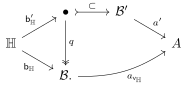
∙; ℬ′; ℍ; A; ℬ.; ⊂; q; a′; 𝖻ℍ′; 𝖻ℍ; a𝗏ℍ

Therefore, Lemma 3.36 implies that

∙; ℬ′; X; ℍ; A; ℬ.; ⊂; q; a′; 𝖻𝕏′; 𝖻𝕏; ξ𝕏; 𝖻ℍ′; 𝖻ℍ; a𝗏ℍ

commutes for any game 𝕏=(X,θ)\mathbb{X}=(X,\theta). This completes the proof of Theorem 4.8.

4.2.4. Examples of Bouton monoids

We conclude this section by giving several examples of the Bouton monoids.

Proposition 4.14 (A categorical characterization of Nim-sum).

The monoid of nim-sum (ℕ,0,⊕)(\mathbb{N},0,\oplus) is isomorphic to the Bouton monoid ℬ+,𝖮𝗎𝗍𝖼𝗈𝗆𝖾\mathcal{B}_{{+},\mathsf{Outcome}} of the Conway addition +{+} and the outcome 𝖮𝗎𝗍𝖼𝗈𝗆𝖾\mathsf{Outcome}.

Example 4.15 (ℬ∨,𝖮𝗎𝗍𝖼𝗈𝗆𝖾\mathcal{B}_{\lor,\mathsf{Outcome}}).

The Bouton monoid ℬ∨,𝖮𝗎𝗍𝖼𝗈𝗆𝖾\mathcal{B}_{\lor,\mathsf{Outcome}} of the selective sum (Example 4.3) and the outcome is given by ℬ∨,𝖮𝗎𝗍𝖼𝗈𝗆𝖾={P,N}\mathcal{B}_{\lor,\mathsf{Outcome}}=\{P,N\} as essentially pointed out in [Smi66]. The binary operation ℬ∨,𝖮𝗎𝗍𝖼𝗈𝗆𝖾×ℬ∨,𝖮𝗎𝗍𝖼𝗈𝗆𝖾→ℬ∨,𝖮𝗎𝗍𝖼𝗈𝗆𝖾\mathcal{B}_{\lor,\mathsf{Outcome}}\times\mathcal{B}_{\lor,\mathsf{Outcome}}\to\mathcal{B}_{\lor,\mathsf{Outcome}} is given by min\min with respect to the order N<PN<P.

Example 4.16 (ℬ∧,𝖮𝗎𝗍𝖼𝗈𝗆𝖾\mathcal{B}_{\land,\mathsf{Outcome}}).

The Bouton monoid of the conjunctive sum ∧\land (Example 4.4) and the outcome 𝖮𝗎𝗍𝖼𝗈𝗆𝖾\mathsf{Outcome} is known to be remoteness ([Smi66]).

ℬ∧,𝖮𝗎𝗍𝖼𝗈𝗆𝖾={P2​k∣k∈ℕ}∪{N2​k+1∣k∈ℕ}\mathcal{B}_{\land,\mathsf{Outcome}}=\{P_{2k}\mid k\in\mathbb{N}\}\cup\{N_{2k+1}\mid k\in\mathbb{N}\}

Here, as the considered monoidal structure ∧\land is non-unital, the resulting Bouton “monoid” ℬ∧,𝖮𝗎𝗍𝖼𝗈𝗆𝖾\mathcal{B}_{\land,\mathsf{Outcome}} is also non-unital, i.e., it is just a semigroup (Remark 4.1). In fact, the binary operation is given by min\min with respect to the order P0<N1<P2<N3<P4<…P_{0}<N_{1}<P_{2}<N_{3}<P_{4}<\dots, which does not admit a neutral element. The minimality of the Bouton monoid can be checked by considering ElM\mathrm{ElM} (Example 2.7, Example C.3).

An example of a game-theoretically motivated Boouton monoid whose target game value is not 𝖮𝗎𝗍𝖼𝗈𝗆𝖾\mathsf{Outcome} is mentioned in Section 5.4.2 (without being able to give an explicit description).

5. Concluding remarks and open questions

As there are still a lot of things to be calculated, we list some of the remaining questions with related observations.

5.1. The Missing Piece: differential structures of games

While our paper defined the Bouton monoid and described an abstruct construction (Section 4.2), there remains the crucial part — the concrete construction of the Bouton monoid. For example, the proof of Proposition 4.14 relies on Theorem 2.17. In that sense, it remains unsatisfactory as a true “demystification” of the nim-sum.

What we should demystify is the proof of Theorem 2.17. The only non-trivial part of the proof is the following equation regarding the nim-sum ⊕\oplus and the mex operator:

(6) ∀S,T∈𝒫fin​(ℕ),𝗆𝖾𝗑⁡(S)⊕𝗆𝖾𝗑⁡(T)=𝗆𝖾𝗑⁡(S⊕𝗆𝖾𝗑⁡(T)∪𝗆𝖾𝗑⁡(S)⊕T),\forall S,T\in\mathcal{P}_{\mathrm{fin}}(\mathbb{N}),\;\mathsf{mex}(S)\oplus\mathsf{mex}(T)=\mathsf{mex}(S\oplus\mathsf{mex}(T)\cup\mathsf{mex}(S)\oplus T),

where we adopt the notion n⊕S≔{n⊕s∣s∈S}n\oplus S\coloneqq\{n\oplus s\mid s\in S\} for n∈ℕn\in\mathbb{N} and S∈𝒫fin​(ℕ)S\in\mathcal{P}_{\mathrm{fin}}(\mathbb{N}). Furthermore, this equation recursively determines the value of the nim-sum since n⊕mn\oplus m is deteremined by choosing S={0,1,…,n−1}S=\{0,1,\dots,n-1\} and T={0,1,…,m−1}T=\{0,1,\dots,m-1\}.

The equation (Equation 6) is reminiscent of the integral version of the Leibniz rule, called the Rota-Baxter equation

∫f×∫g=∫(f×∫g+∫f×g)\textstyle\int f\times\int g=\int\left(f\times\int g+\int f\times g\right)

by regarding the sets S,TS,T as functions, ⊕\oplus as products, and 𝗆𝖾𝗑\mathsf{mex} as integration. This “Rota-Baxter equation” of the nim-sum is a reflection of a more trivial “Leibniz rule” of the Conway addition:

θ𝕏+𝕐​(x,y)=θ𝕏​(x)×{y}∪{x}×θ𝕐​(y),\theta_{\mathbb{X}+\mathbb{Y}}(x,y)=\theta_{\mathbb{X}}(x)\times\{y\}\cup\{x\}\times\theta_{\mathbb{Y}}(y),

which resembles the genuine Leibniz rule ∂(f×g)=∂f×g+f×∂g\partial(f\times g)=\partial f\times g+f\times\partial g. Note that we see here a kind of the twistedness in Diagram 3 as the “differential part” θ\theta goes in the opposite direction of the “integral part” 𝗆𝖾𝗑\mathsf{mex}.

Expecting the remaining equation (Equation 6) is actually a reflection of some differential structure on (𝐆𝐚𝐦𝐞,+)(\mathbf{Game},+), we ask the first question.

Question 5.1.

How do these “differential structures” appear in our formulation, especially for the Bouton monoids ℬ𝗏,+\mathcal{B}_{\mathsf{v},+} with respect to the Conway addition?

Let us describe a partial solution to this question:

Proposition 5.2 (Rota-Baxter equation for the Bouton monoids w.r.t. the Conway addition).

Let 𝗏\mathsf{v} be a game value. If the Bouton monoid {𝖻𝕏:X→ℬ𝗏,+}𝕏=(X,θ): game\{\mathsf{b}_{\mathbb{X}}\colon X\to\mathcal{B}_{\mathsf{v},+}\}_{\mathbb{X}=(X,\theta):\text{ game}} of 𝗏\mathsf{v} with respect to the Conway addition ++ is induced by a 𝒫fin\mathcal{P}_{\mathrm{fin}}-algebra structure (ℬ𝗏,+,β:𝒫fin(ℬ𝗏,+)→ℬ𝗏,+)(\mathcal{B}_{\mathsf{v},+},\beta\colon\mathcal{P}_{\mathrm{fin}}(\mathcal{B}_{\mathsf{v},+})\to\mathcal{B}_{\mathsf{v},+}), then the monoid structure ⊛:ℬ𝗏,+×ℬ𝗏,+→ℬ𝗏,+\circledast\colon\mathcal{B}_{\mathsf{v},+}\times\mathcal{B}_{\mathsf{v},+}\to\mathcal{B}_{\mathsf{v},+} satisfies the following Rota-Baxter equation:

β⁡(S)⊛β⁡(T)=β⁡(S⊛β⁡(T)∪β⁡(S)⊛T)\beta(S)\circledast\beta(T)=\beta(S\circledast\beta(T)\cup\beta(S)\circledast T)

for any S,T∈𝒫fin​(ℬ𝗏,+)S,T\in\mathcal{P}_{\mathrm{fin}}(\mathcal{B}_{\mathsf{v},+}).

Proof.

In this proof, the image of a subset S⊂XS\subset X by a function f:X→Yf\colon X\to Y is denoted by f⁡[S]⊂Yf[S]\subset Y. Since the function 𝖻ℍ:ℍ→ℬ𝗏,+\mathsf{b}_{\mathbb{H}}\colon\mathbb{H}\to\mathcal{B}_{\mathsf{v},+} is surjective by the consturction, for any S,T∈𝒫fin​(ℬ𝗏,+)S,T\in\mathcal{P}_{\mathrm{fin}}(\mathcal{B}_{\mathsf{v},+}), we can take A,B∈𝒫fin​(ℍ)A,B\in\mathcal{P}_{\mathrm{fin}}(\mathbb{H}) such that 𝖻ℍ​[A]=S\mathsf{b}_{\mathbb{H}}[A]=S and 𝖻ℍ​[B]=T\mathsf{b}_{\mathbb{H}}[B]=T. By the assmption that the game value 𝖻\mathsf{b} is induced by a 𝒫fin\mathcal{P}_{\mathrm{fin}}-algebra structure (ℬ𝗏,+,β:𝒫fin(ℬ𝗏,+)→ℬ𝗏,+)(\mathcal{B}_{\mathsf{v},+},\beta\colon\mathcal{P}_{\mathrm{fin}}(\mathcal{B}_{\mathsf{v},+})\to\mathcal{B}_{\mathsf{v},+}), we have 𝖻𝕏​(x)=β⁡(𝖻𝕏​[θ𝕏​(x)])\mathsf{b}_{\mathbb{X}}(x)=\beta(\mathsf{b}_{\mathbb{X}}[\theta_{\mathbb{X}}(x)]), in particular, we have 𝖻ℍ​(A)=β⁡(𝖻ℍ​[A])=β⁡(S)\mathsf{b}_{\mathbb{H}}(A)=\beta(\mathsf{b}_{\mathbb{H}}[A])=\beta(S) and 𝖻ℍ​(B)=β​(T)\mathsf{b}_{\mathbb{H}}(B)=\beta(T). As 𝖻ℍ\mathsf{b}_{\mathbb{H}} is a monoid homomorphism by the construction, we have

𝖻ℍ(A)⊛𝖻ℍ(B)=𝖻ℍ(A+ℍB).\mathsf{b}_{\mathbb{H}}(A)\circledast\mathsf{b}_{\mathbb{H}}(B)=\mathsf{b}_{\mathbb{H}}(A+_{\mathbb{H}}B).

The left-hand side is equal to β⁡(S)⊛β⁡(T)\beta(S)\circledast\beta(T). The right-hand side is calculated as

𝖻ℍ(A+ℍB)=\displaystyle\mathsf{b}_{\mathbb{H}}(A+_{\mathbb{H}}B)= β(𝖻ℍ[{a+ℍB∣a∈A}∪{A+ℍb∣b∈B}])\displaystyle\beta\left(\mathsf{b}_{\mathbb{H}}[\{a+_{\mathbb{H}}B\mid a\in A\}\cup\{A+_{\mathbb{H}}b\mid b\in B\}]\right)
=\displaystyle= β({𝖻ℍ(a+ℍB)∣a∈A}∪{𝖻ℍ(A+ℍb)∣b∈B})\displaystyle\beta(\{\mathsf{b}_{\mathbb{H}}(a+_{\mathbb{H}}B)\mid a\in A\}\cup\{\mathsf{b}_{\mathbb{H}}(A+_{\mathbb{H}}b)\mid b\in B\})
=\displaystyle= β⁡({𝖻ℍ​(a)⊛𝖻ℍ​(B)∣a∈A}∪{𝖻ℍ​(A)⊛𝖻ℍ​(b)∣b∈B})\displaystyle\beta(\{\mathsf{b}_{\mathbb{H}}(a)\circledast\mathsf{b}_{\mathbb{H}}(B)\mid a\in A\}\cup\{\mathsf{b}_{\mathbb{H}}(A)\circledast\mathsf{b}_{\mathbb{H}}(b)\mid b\in B\})
=\displaystyle= β⁡(𝖻ℍ​[A]⊛𝖻ℍ​(B)∪𝖻ℍ​(A)⊛𝖻ℍ​[B])\displaystyle\beta(\mathsf{b}_{\mathbb{H}}[A]\circledast\mathsf{b}_{\mathbb{H}}(B)\cup\mathsf{b}_{\mathbb{H}}(A)\circledast\mathsf{b}_{\mathbb{H}}[B])
=\displaystyle= β⁡(S⊛β⁡(T)∪β⁡(S)⊛T).\displaystyle\beta(S\circledast\beta(T)\cup\beta(S)\circledast T).

This completes the proof. ∎

5.2. Partisan games

What we called games in this paper is usually called impartial games. We intentionally choose to concentrate on impartial games since our central motivation is to demystify the nim-sum. However, in many different contexts, partisam games, games in which a Left-player and a Right-player have different options, are of interest.

Instead of considering 𝒫fin:𝐒𝐞𝐭→𝐒𝐞𝐭\mathcal{P}_{\mathrm{fin}}\colon\mathbf{Set}\to\mathbf{Set}, we can alternatively consider 𝒫fin×𝒫fin:𝐒𝐞𝐭→𝐒𝐞𝐭\mathcal{P}_{\mathrm{fin}}\times\mathcal{P}_{\mathrm{fin}}\colon\mathbf{Set}\to\mathbf{Set} to obtain the parallel theory of “partisan games as reursive coalgebras” and to mimick all the abstract nonsenses we used in this paper. (A similar idea of using coalgebras of 𝒫×𝒫\mathcal{P}\times\mathcal{P} to study partisan games has already appeared in [HL09].)

Question 5.3.

To which extent the theory of partisan games are comprehended by replacing 𝒫fin\mathcal{P}_{\mathrm{fin}} by 𝒫fin×𝒫fin\mathcal{P}_{\mathrm{fin}}\times\mathcal{P}_{\mathrm{fin}}?

For example, we can capture the definition of (short and partisan) Conway games, which is recursively defined as a pair of finite sets of Conway games, as follows:

Proposition 5.4.

The terminal recursive 𝒫fin×𝒫fin\mathcal{P}_{\mathrm{fin}}\times\mathcal{P}_{\mathrm{fin}}-coalgebra is given by the set 𝔾\mathbb{G} of all (short and partisan) Conway games.

5.3. Classification problem of monoidal structures

In order to fathom the applicativity of Theorem 4.8, we would like to classify monoidal structures on 𝐆𝐚𝐦𝐞\mathbf{Game}. The first question to be asked is the most restrictive one:

Question 5.5.

Classify all symmetric mononoidal closed structures on 𝐆𝐚𝐦𝐞\mathbf{Game} such that U:𝐆𝐚𝐦𝐞→𝐒𝐞𝐭U\colon\mathbf{Game}\to\mathbf{Set} is strictly monoidal.

Notice that the closedness assumption is redundant due to Corollary B.11. A similar research has been recently done for graphs [KK24]. See also [FLK80].

If there are infinitely many examples, we obtain infinitely many applications of Theorem 4.8, and if there are only finitely many examples, we obtain a finite list of all “nicely behaved notions of game-sums,” which may be of independent interest.

As Theorem 4.8 works also for a non-unital monoidal structure, the loosest classification problem regarding Theorem 4.8 is the following one.

Question 5.6.

Classify all non-unital mononoidal structures on 𝐆𝐚𝐦𝐞\mathbf{Game} such that U:𝐆𝐚𝐦𝐞→𝐒𝐞𝐭U\colon\mathbf{Game}\to\mathbf{Set} is lax monoidal.

5.4. Other questions

In the rest of this section, we will list some problems, which might be of interest for some readers.

5.4.1. The closed structure

One can check that the Conway addition structure is symmetric monoidal closed (Corollary B.11) by an anstract argument.

Question 5.7 (The closed structure).

What is the internal hom with respect to the Conway addition?

In the classical context (including [Joy77]), the closedness plays the key role of switching the two players. It makes their category of games compact closed, which categorifies the classical ordered abelian group of Conway games! The closed structure might be better understood when we consider the partisan games 𝐑𝐞𝐜𝐂𝐨𝐚𝐥𝐠𝒫fin×𝒫fin\mathbf{RecCoalg}_{\mathcal{P}_{\mathrm{fin}}\times\mathcal{P}_{\mathrm{fin}}} (see Section 5.2).

5.4.2. Other types of Bouton monoid: towards circular nim

One of the motivating phenomena of this research is an open problem in combinatorial game theory: the circular nim [DH13]. In circular nim CN⁡(n,k)\mathrm{CN}(n,k) for 0<k≤n0<k\leq n, nn piles are arranged on a circle. At each move, a player selects kk consecutive piles and removes a total of at least one stone from them. The winning strategy for CN⁡(6,2)\mathrm{CN}(6,2) remains an open question [DH13, Section 3].
a1; a2; a3; a4; a5; a6
Figure 14. Circular nim

But how is CN⁡(6,2)\mathrm{CN}(6,2) related to the Bouton monoid? By an easy argument, one can observe that CN⁡(6,2)\mathrm{CN}(6,2) contains Nim1+(Nim1∨(Nim1+Nim1))\mathrm{Nim}_{1}+(\mathrm{Nim}_{1}\lor(\mathrm{Nim}_{1}+\mathrm{Nim}_{1})) as its subgame.

Nim1+(Nim1∨(Nim1+Nim1))\displaystyle\mathrm{Nim}_{1}+(\mathrm{Nim}_{1}\lor(\mathrm{Nim}_{1}+\mathrm{Nim}_{1})) ↣CN⁡(6,2)\displaystyle\rightarrowtail\mathrm{CN}(6,2)
(a1,a4,a3,a5)\displaystyle(a_{1},a_{4},a_{3},a_{5}) ↦(a1,0,a3,a4,a5,0)\displaystyle\mapsto(a_{1},0,a_{3},a_{4},a_{5},0)

Therefore, as a subproblem of CN⁡(6,2)\mathrm{CN}(6,2), we need to understand the winning strategy of Nim1+(Nim1∨(Nim1+Nim1))\mathrm{Nim}_{1}+(\mathrm{Nim}_{1}\lor(\mathrm{Nim}_{1}+\mathrm{Nim}_{1})), which also remains an open question, to the best of the author’s knowledge. In order to decompose the nested structure of the game, one naïve idea is to understand the nested Bouton monoid

ℬ∨,ℬ+,𝖮𝗎𝗍𝖼𝗈𝗆𝖾=ℬ∨,𝖦𝗋𝗎𝗇𝖽𝗒.\mathcal{B}_{\lor,\mathcal{B}_{+,\mathsf{Outcome}}}=\mathcal{B}_{\lor,\mathsf{Grundy}}.
Question 5.8.

What is the Bouton monoid ℬ∨,𝖦𝗋𝗎𝗇𝖽𝗒\mathcal{B}_{\lor,\mathsf{Grundy}}? Is it just the miniture monoid (ℍ,∨ℍ)(\mathbb{H},\lor_{\mathbb{H}})?

If it is a proper quotient of (ℍ,∨ℍ)(\mathbb{H},\lor_{\mathbb{H}}), it might be a useful tool to tackle CN⁡(6,2)\mathrm{CN}(6,2); otherwise, it at least captures one mathematical aspect of the difficulty of CN⁡(6,2)\mathrm{CN}(6,2). Let us say a game value 𝗏\mathsf{v} is essentially indecomposable by a monoidal structure ∗\ast if 𝖻ℍ:ℍ→ℬ∗,𝗏\mathsf{b}_{\mathbb{H}}\colon\mathbb{H}\to\mathcal{B}_{\ast,\mathsf{v}} is bijective. Then, we can ask: is the Grundy number essentially indecomposable by the selective sum? This kind of question might serve as a passive approach to a difficult game in order to mathematically state one aspect of its difficulty.

5.4.3. Other endofunctors

In this paper, we have concentrated on the endofunctor 𝒫fin:𝐒𝐞𝐭→𝐒𝐞𝐭\mathcal{P}_{\mathrm{fin}}\colon\mathbf{Set}\to\mathbf{Set} by restraining our categorical desire to generalize it. As we used only simple abstract nonsense, our argument should be able to be categorically generalized.

Question 5.9.

To what extent is our framework categorically generalized? In particular, can it be done for any locally presentable category 𝒞\mathcal{C} and any accessible endofunctor T:𝒞→𝒞T\colon\mathcal{C}\to\mathcal{C}?

This question is of not only categorical interest but also game-theoretic interest. As explained in Section 5.2, 𝒫fin×𝒫fin:𝐒𝐞𝐭→𝐒𝐞𝐭\mathcal{P}_{\mathrm{fin}}\times\mathcal{P}_{\mathrm{fin}}\colon\mathbf{Set}\to\mathbf{Set} is another (possibly the most important) example. We are also interested in other variants like multiplayer games, probabilistic games, linear games, and transfinite games.

Appendix A Existence of the minimum monoid factorizations

In this appendix, we will explain the context and the construction of the minimum monoid factorization (Definition 4.13).

Proposition A.1 (Unique existence and the construction).

For any monoid MM, any set AA, and any function f:M→Af\colon M\to A, its minimum monoid factorization f:M→qfMf→afAf\colon M\xrightarrow{q_{f}}M_{f}\xrightarrow{a_{f}}A uniquely exists up to a canonical isomorphism. Furthermore, the monoid homomorphism qf:M→Mfq_{f}\colon M\to M_{f} is surjective, and the corresponding monoid congruence ∼f={(m,m′)∈M×M∣qf(m)=qf(m′)}⊂M×M{\sim_{f}}=\{(m,m^{\prime})\in M\times M\mid q_{f}(m)=q_{f}(m^{\prime})\}\subset M\times M is given by

m∼fm′⇔for any a,b∈M,f(amb)=f(am′b).m\sim_{f}m^{\prime}\iff\textrm{for any }a,b\in M,f(amb)=f(am^{\prime}b).
Proof.

First, we need to prove that the equivalence relation ∼f\sim_{f} is a monoid congruence. If m∼fm′m\sim_{f}m^{\prime} and n∼fn′n\sim_{f}n^{\prime}, we have

f⁡(a​m​n​b)=f⁡(a​m′​n​b)=f⁡(a​m′​n′​b)f(amnb)=f(am^{\prime}nb)=f(am^{\prime}n^{\prime}b)

for any a,b∈Ma,b\in M, and thus mn∼fm′n′mn\sim_{f}m^{\prime}n^{\prime}. This proves that ∼f\sim_{f} is a monoid congruence, and thus the monoid structure on M/∼fM/{\sim_{f}} and a surjective monoid homomorphism qf:M↠Mf≔M/∼fq_{f}\colon M\twoheadrightarrow M_{f}\coloneqq M/{\sim_{f}} are well-defined. Furthermore, the function af:Mf→A:[m]∼f↦f(m)a_{f}\colon M_{f}\to A:[m]_{\sim_{f}}\mapsto f(m) is also well-defined because we have m∼fm′⟹f(m)=f(m′)m\sim_{f}m^{\prime}\implies f(m)=f(m^{\prime}) by taking the neutral element as a,ba,b.

So far, we have obtained a factorization f:M→qfMf→afAf\colon M\xrightarrow{q_{f}}M_{f}\xrightarrow{a_{f}}A. We prove the minimality. Let us take a monoid Mf′M^{\prime}_{f} equipped with a factorization f=M→qf′Mf′→af′Af=M\xrightarrow{q^{\prime}_{f}}M^{\prime}_{f}\xrightarrow{a^{\prime}_{f}}A into a monoid homomorphism qf′:M→Mf′q^{\prime}_{f}\colon M\to M^{\prime}_{f} followed by a function af′:Mf′→Aa^{\prime}_{f}\colon M^{\prime}_{f}\to A. Then we prove that there exsits a surjective monoid homomorphism q:Im⁡(qf′)↠Mfq\colon\mathrm{Im}(q^{\prime}_{f})\twoheadrightarrow M_{f} from the submonoid Im⁡(qf′)⊂Mf′\mathrm{Im}(q^{\prime}_{f})\subset M^{\prime}_{f} such that the following diagram commutes.
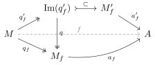
Im⁡(qf′); Mf′; M; A; Mf; ⊂; q; af′; f; qf′; qf; af

As both qf:M↠Mfq_{f}\colon M\twoheadrightarrow M_{f} and qf′:M↠Im⁡(qf′)q^{\prime}_{f}\colon M\twoheadrightarrow\mathrm{Im}(q^{\prime}_{f}) are surjective monoid homomorphisms, if a function q:Im⁡(qf′)→Mfq\colon\mathrm{Im}(q^{\prime}_{f})\to M_{f} that makes the left triangle commutative exsits, then it automatically follows that the function qq is also a surjective monoid homomorphism, and that the right-hand side skew rectangle is also commutative. So it suffices to prove the implication qf′(m)=qf′(m′)⟹m∼fm′q^{\prime}_{f}(m)=q^{\prime}_{f}(m^{\prime})\implies m\sim_{f}m^{\prime} for any m,m′∈Mm,m^{\prime}\in M. If qf′​(m)=qf′​(m′)q^{\prime}_{f}(m)=q^{\prime}_{f}(m^{\prime}), then for any a,b∈Ma,b\in M, we have qf′​(a​m​b)=qf′​(a)​qf′​(m)​qf′​(b)=qf′​(a)​qf′​(m′)​qf′​(b)=qf′​(a​m′​b)q^{\prime}_{f}(amb)=q^{\prime}_{f}(a)q^{\prime}_{f}(m)q^{\prime}_{f}(b)=q^{\prime}_{f}(a)q^{\prime}_{f}(m^{\prime})q^{\prime}_{f}(b)=q^{\prime}_{f}(am^{\prime}b), hence f⁡(a​m​b)=f⁡(a​m′​b)f(amb)=f(am^{\prime}b). This proves the implication qf′(m)=qf′(m′)⟹m∼fm′q^{\prime}_{f}(m)=q^{\prime}_{f}(m^{\prime})\implies m\sim_{f}m^{\prime} and completes the proof. ∎

The structure of the minimum quotient is by no means anything nontrivial nor advanced – the idea of “minimizing an algebraic structure without losing too much information” is quite mundane as exemplified by the following examples.

Example A.2 (Real numbers in complex numbers).

If you care whether the sum of two complex numbers is real, then it suffices to just keep track of the imaginary parts. This obvious fact can be described as follows. Consider a function f:ℂ→{⊤,⊥}f\colon\mathbb{C}\to\{\top,\bot\} defined by

f⁡(z)={⊤(z∈ℝ)⊥(z∉ℝ).f(z)=\begin{cases}\top&(z\in\mathbb{R})\\ \bot&(z\notin\mathbb{R}).\end{cases}

Then, the minimum monoid factorization of ff (with respect to the additive structure of ℂ\mathbb{C}) is given by taking the imaginary part ℂ↠ℝ​i→{⊤,⊥}\mathbb{C}\twoheadrightarrow\mathbb{R}i\to\{\top,\bot\}.

Example A.3 (Syntactic monoid of a languege).

For a finite set Σ\Sigma, a language LL is just a subset of the free monoid L⊂Σ∗L\subset\Sigma^{*}. The syntactic monoid of the language LL is defined as the minimum monoid factorization of the corresponding characteristic function χL:Σ∗→{⊤,⊥}\chi_{L}\colon\Sigma^{*}\to\{\top,\bot\}. See some textbooks on the formal language theory, for example [Pin22], for more details on the syntactic monoids.

Remark A.4 (Minimum 𝕋\mathbb{T}-algebra factorization).

Actually, any equational theory 𝕋\mathbb{T} admits the property like Proposition A.1. In fact, for any 𝕋\mathbb{T}-algebra AA, the complete lattice of 𝕋\mathbb{T}-algebra congruences is a complete sublattice of the complete lattice of equivalence relations on the underlying set AA

Congruence𝕋​(A)↪Equiv⁡(A),\mathrm{Congruence}_{\mathbb{T}}(A)\hookrightarrow\mathrm{Equiv(A)},

which is known in the universal algebra theory ([BS81, II Theorem 5.3]). Due to the adjoint functor theorem, the embedding admits both left and right adjoint, and the right adjoint part provides the desired minimum 𝕋\mathbb{T}-algebra factorization. In particular, we have the minimum subgroup factorization, which we need in the context of Remark 4.1.

Remark A.5.

The construction of the minimum monoid factorization is ubiquitous in combinatorial game theory. For example, even the “equality” of games is conventionally defined in this way! See [Sie13].

Appendix B Categorical properties of 𝐆𝐚𝐦𝐞\mathbf{Game}

In this appendix, we study the categorical properties of 𝐆𝐚𝐦𝐞\mathbf{Game} and prove Theorem 3.15:

Theorem B.9:

The category of games 𝐆𝐚𝐦𝐞\mathbf{Game} is locally finitely presentable. In particular, it has all small limits and colimits.

Proposition B.23:

The forgetful functor U:𝐆𝐚𝐦𝐞→𝐒𝐞𝐭U\colon\mathbf{Game}\to\mathbf{Set} is comonadic. In particular, it preserves, reflects, and strictly creates all small colimits.

Proposition B.26:

The category of games 𝐆𝐚𝐦𝐞\mathbf{Game} has a subobject classifier.

We will also prove that

Corollary B.19:

The category of games 𝐆𝐚𝐦𝐞\mathbf{Game} has the epi-mono orthogonal factorization system.

Remark B.27:

The category of games 𝐆𝐚𝐦𝐞\mathbf{Game} is not cartesian closed. In particular, it is not a topos.

Remark B.1 (Comparison with locally finite Kripke frames).

In [DG24], the categorical properties of the category of Kripke frames 𝐊𝐅𝐫≃𝐂𝐨𝐚𝐥𝐠𝒫\mathbf{KFr}\simeq\mathbf{Coalg}_{\mathcal{P}} are studied, and then the category of locally finite Kripke frames 𝐊𝐅𝐫l​f\mathbf{KFr}_{lf} is studied in the context of the duality in modal logic. As our category of games 𝐆𝐚𝐦𝐞\mathbf{Game} is a full subcategory of 𝐊𝐅𝐫l​f\mathbf{KFr}_{lf}, some arguments in this appendix already appeared in [DG24]. For example, game morphisms correspond to [DG24, Definition 3.3], subgames (Definition B.3) to generated subframe [DG24, Definition 3.7], the descripton of colimits to [DG24, Proposition 3.9], the description of the equalizer to [DG24, Lemma 3.11], the local presentability to [DG24, Theorem 4.3], and the comonadicity to [DG24, Theorem 5.4].

𝐑𝐞𝐜𝐂𝐨𝐚𝐥𝐠𝒫fin≃𝐆𝐚𝐦𝐞⊊𝐊𝐅𝐫l​f⊊𝐊𝐅𝐫≃𝐂𝐨𝐚𝐥𝐠𝒫\mathbf{RecCoalg}_{\mathcal{P}_{\mathrm{fin}}}\simeq\mathbf{Game}\subsetneq\mathbf{KFr}_{lf}\subsetneq\mathbf{KFr}\simeq\mathbf{Coalg}_{\mathcal{P}}

B.1. 𝐆𝐚𝐦𝐞\mathbf{Game} is locally finitely presentable

We will prove that the category 𝐆𝐚𝐦𝐞\mathbf{Game} is locally finitely presentable. For those who are not familiar with presentability, the standard textbook is [AR94]. Our proof of the local presentability is very similar to that of [DG24]. As we will check the definition naïvely, we need to know the colimits in 𝐆𝐚𝐦𝐞\mathbf{Game} first.

Lemma B.2.

The forgetful functor U:𝐆𝐚𝐦𝐞→𝐒𝐞𝐭U\colon\mathbf{Game}\to\mathbf{Set} strictly creates all small colimits. In particular, 𝐆𝐚𝐦𝐞\mathbf{Game} is cocomplete and UU preserves and reflects them. Furthermore, UU is conservative.

Proof.

The forgetful functor is decomposed into the two forgetful functors

𝐆𝐚𝐦𝐞→U0𝐂𝐨𝐚𝐥𝐠𝒫fin→U1𝐒𝐞𝐭.\mathbf{Game}\xrightarrow{U_{0}}\mathbf{Coalg}_{\mathcal{P}_{\mathrm{fin}}}\xrightarrow{U_{1}}\mathbf{Set}.

The first one U0:𝐆𝐚𝐦𝐞→𝐂𝐨𝐚𝐥𝐠𝒫finU_{0}\colon\mathbf{Game}\to\mathbf{Coalg}_{\mathcal{P}_{\mathrm{fin}}} is fully faithful, and admits a right adjoint of taking the well-founded part ([AMM20, Proposition 4.19]). Therefore, 𝐆𝐚𝐦𝐞\mathbf{Game} is coreflective subcategory of 𝐂𝐨𝐚𝐥𝐠𝒫fin\mathbf{Coalg}_{\mathcal{P}_{\mathrm{fin}}} and the embedding functor U0U_{0} is conservative and creates all small colimits. The other one U1:𝐂𝐨𝐚𝐥𝐠𝒫fin→𝐒𝐞𝐭U_{1}\colon\mathbf{Coalg}_{\mathcal{P}_{\mathrm{fin}}}\to\mathbf{Set} is conservative and creates all small colimits by the general theory of coalgebras of an endofunctor. ∎

Definition B.3 (Subgame).

A subgame of a game 𝕏=(X,→)\mathbb{X}=(X,\to) is a subset S⊂XS\subset X such that if x∈Sx\in S and x→x′x\to x^{\prime} then x′∈Sx^{\prime}\in S.

As we will see later, subgames are almost the same as monomorphisms (Proposition B.18).

Lemma B.4 (Image is a subgame).

For a game morphism f:𝕏→𝕐f\colon\mathbb{X}\to\mathbb{Y}, its image Im​f\mathrm{Im}{f} is a subgame of 𝕐\mathbb{Y}.

Proof.

This is due to the path-lifting condition of Definition 3.12. ∎

For any injective game morphism f:𝕐→𝕏f\colon\mathbb{Y}\to\mathbb{X}, its image Im⁡(f)\mathrm{Im}(f) is isomorphic to 𝕐\mathbb{Y} as games since UU is conservative (Lemma B.2). Therefore, by abuse of terminology, we will call an injective game morphism a subgame.

Definition B.5.

For a game 𝕏=(X,→)\mathbb{X}=(X,\to) and a subset S⊂XS\subset X, the minimum subgame of 𝕏\mathbb{X} that contains SS is called the subgame generated by SS.

See Lemma B.21 for its construction.

Lemma B.6.

Any subgame generated by a finite subset is finite.

Proof.

This follows from the two finiteness conditions in the definition of games (Definition 2.1). (cf. Remark 2.4). ∎

Lemma B.7.

Every game is the filtered colimit of (the canonical diagram of) its finite subgames.

Proof.

For any finite subset S⊂XS\subset X of a game 𝕏=(X,θ)\mathbb{X}=(X,\theta), the minimum subgame containing SS is finite. Therefore the canonical diagram is in fact filtered, and Lemma B.2 completes the proof. ∎

Lemma B.8 (Finitely presentable == Finite).

A game 𝕏=(X,θ)\mathbb{X}=(X,\theta) is finitely presentable if and only if its underlying set XX is finite.

Proof.

Let us take an arbitrary game 𝕏=(X,θ)\mathbb{X}=(X,\theta). If a game 𝕏\mathbb{X} is finitely presentable, Lemma B.7 implies that 𝕏\mathbb{X} coincides with its finite subgame, and hence XX itself is finite.

Conversely, assuming that the underlying set XX is finite, we will prove that the hom functor

𝐆𝐚𝐦𝐞⁡(𝕏,−):𝐆𝐚𝐦𝐞→𝐒𝐞𝐭\mathbf{Game}(\mathbb{X},-)\colon\mathbf{Game}\to\mathbf{Set}

preserves filtered colimits.

Let 𝒞\mathcal{C} be a filtered category, F:𝒞→𝐆𝐚𝐦𝐞F\colon\mathcal{C}\to\mathbf{Game} be a functor, and {αc:F​c→𝕐}c∈ob​𝒞\{\alpha_{c}\colon Fc\to\mathbb{Y}\}_{c\in\mathrm{ob}{\mathcal{C}}} be the colimit cocone. Take an arbitrary morphism f:𝕏→𝕐f\colon\mathbb{X}\to\mathbb{Y}. Our goal is to prove that there exists c∈ob​𝒞c\in\mathrm{ob}{\mathcal{C}} such that ff has a lift gg along αc\alpha_{c}

Fc; 𝕏; 𝕐.; αc; f; ∃g

(The essential uniqueness of the factorization follows from the case of 𝐒𝐞𝐭\mathbf{Set} and Lemma B.2.)

Since a finite set is finitely presentable in 𝐒𝐞𝐭\mathbf{Set}, and UU preserves small colimits (in particuler, filtered colimits), there exists a function h:U​𝕏→U​F​ch\colon U\mathbb{X}\to UFc such that the following diagram commutes
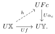
UFc; U𝕏; U𝕐.; Uαc; Uf; h

Let ι:𝕊→F​c\iota\colon\mathbb{S}\to Fc be the subgame of F​cFc, generated by the image of hh. Since 𝕏\mathbb{X} is finite, 𝕊\mathbb{S} is also finite (Lemma Lemma B.6). So far, we have onbtained the diagram
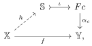
𝕊; Fc; 𝕏; 𝕐,; ι; αc; f; h

where hh is denoted by a dashed arrow since it is a mere function. Since 𝕐\mathbb{Y} is a filtered colimit (preserved by UU) and 𝕊\mathbb{S} is finite, there exists k:c→c′k\colon c\to c^{\prime} in 𝒞\mathcal{C} such that αc′\alpha_{c^{\prime}} is injective on the subgame F​k​(𝕊)=Im⁡(F​k∘ι)Fk(\mathbb{S})=\mathrm{Im}{(Fk\circ\iota)} of F​c′Fc^{\prime} (Lemma B.4). In other words, the morphism αc′∘m\alpha_{c^{\prime}}\circ m in the following diagram is injective.
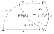
𝕊; Fc; Fk(𝕊); Fc′; 𝕏; 𝕐,; ι; e; αc; Fk; m; αc′∘m; αc′; f; h

Because the morphism αc′∘m\alpha_{c^{\prime}}\circ m is injective, the game F​k​(𝕊)Fk(\mathbb{S}) can be regarded as a subgame of 𝕐\mathbb{Y}. Therefore, the composite e∘fe\circ f, which is the lift of ff along αc′∘m\alpha_{c^{\prime}}\circ m, is a game morphism

𝕊; Fc; Fk(𝕊); Fc′; 𝕏; 𝕐.; ι; e; αc; Fk; m; αc′∘m; αc′; f; e∘h; h

This proves that ff has a lift along αc′\alpha_{c^{\prime}} in the category 𝐆𝐚𝐦𝐞\mathbf{Game}. ∎

Theorem B.9.

The category of games 𝐆𝐚𝐦𝐞\mathbf{Game} is locally fintiely presentble.

Proof.

We have observed that 𝐆𝐚𝐦𝐞\mathbf{Game} is cocomplete (Lemma B.2) and admits a small number of finitely presentable objects (Lemma B.8), and that every object is a filtered colimit of finitely presentable objects (Lemma B.7). ∎

Although we have spent a whole subsection to prove the existence of the terminal object in Section 3.6, we can prove much more stronger statement now.

Corollary B.10.

The category of games 𝐆𝐚𝐦𝐞\mathbf{Game} is complete.

Proof.

This follows since every locally presentable category is complete. ∎

Corollary B.11.

All the (non-unital or unital) monoidal structure that lifts the cartesian monoidal structure of 𝐒𝐞𝐭\mathbf{Set}
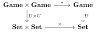
𝐆𝐚𝐦𝐞×𝐆𝐚𝐦𝐞; 𝐆𝐚𝐦𝐞; 𝐒𝐞𝐭×𝐒𝐞𝐭; 𝐒𝐞𝐭; ∗; U×U; U; ×

is monoidal closed.

Proof.

Due to the adjoint functor theorem for locally presentable categories, it suffices to prove that, for any game 𝕏=(X,→)\mathbb{X}=(X,{\to}), the functor 𝕏∗−:𝐆𝐚𝐦𝐞→𝐆𝐚𝐦𝐞\mathbb{X}\ast{-}\colon\mathbf{Game}\to\mathbf{Game} is cocontinuous. This follows from the commutative daigram
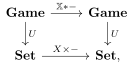
𝐆𝐚𝐦𝐞; 𝐆𝐚𝐦𝐞; 𝐒𝐞𝐭; 𝐒𝐞𝐭,; 𝕏∗−; U; U; X×−

and the fact that the forgetful functor U:𝐆𝐚𝐦𝐞→𝐒𝐞𝐭U\colon\mathbf{Game}\to\mathbf{Set} reflects colimits (Lemma B.2). ∎

This corollary implies that all of the Conway addition (Definition 2.10), the selective sum (Example 4.3), and the conjunctive sum (Example 4.4) are symmetric monoidal closed structure on 𝐆𝐚𝐦𝐞\mathbf{Game}. See also Section 5.4.1.

Corollary B.12.

The forgetful functor U:𝐆𝐚𝐦𝐞→𝐒𝐞𝐭U\colon\mathbf{Game}\to\mathbf{Set} admits a right adjoint.

Proof.

This also follows from the adjoint functor theorem for locally presentable categories and Lemma B.2. ∎

This adjunction is the subject of the next subsection.

B.2. The forgetful ⊣\dashv cofree game adjunction

This subsection aims to describe the right adjoint of the forgetful functor U:𝐆𝐚𝐦𝐞→𝐒𝐞𝐭U\colon\mathbf{Game}\to\mathbf{Set}, which exsits due to Corollary B.12. We temporarily write R:𝐒𝐞𝐭→𝐆𝐚𝐦𝐞R\colon\mathbf{Set}\to\mathbf{Game} for the right adjoint functor and call it the cofree games functor. We already know that R⁡(1)R(1) should be isomorphic to the terminal game ℍ\mathbb{H}. So we write RS=(ℍS,θS:ℍS→𝒫fin(ℍS))RS=(\mathbb{H}_{S},\theta_{S}\colon\mathbb{H}_{S}\to\mathcal{P}_{\mathrm{fin}}(\mathbb{H}_{S})) for the cofree game R​SRS. Let ϵS:U​R​(S)=ℍS→S\epsilon_{S}\colon UR(S)=\mathbb{H}_{S}\to S denote the counit at a set SS.

We will observe that we can calculate ℍS\mathbb{H}_{S} as the initial 𝒫fin​(−)×S\mathcal{P}_{\mathrm{fin}}({-})\times S-algebra and hence by Adamek’s fixed point theorem (cf. Diagram 4)! In fact, we can show that the 𝒫fin​(−)×S\mathcal{P}_{\mathrm{fin}}({-})\times S-coalgebra

(ℍS,⟨θS,ϵS⟩:ℍS→𝒫fin(ℍS)×S)(\mathbb{H}_{S},\langle\theta_{S},\epsilon_{S}\rangle\colon\mathbb{H}_{S}\to\mathcal{P}_{\mathrm{fin}}(\mathbb{H}_{S})\times S)

is the terminal recursive 𝒫fin​(−)×S\mathcal{P}_{\mathrm{fin}}({-})\times S-coalgebra, and hence given by the initial 𝒫fin\mathcal{P}_{\mathrm{fin}}-algebra (Proposition 3.7). Notice that a 𝒫fin​(−)×S\mathcal{P}_{\mathrm{fin}}({-})\times S-coalgebra ⟨θ,σ⟩:X→𝒫fin​(X)×S\langle\theta,\sigma\rangle\colon X\to\mathcal{P}_{\mathrm{fin}}(X)\times S is recursive if and only if the 𝒫fin\mathcal{P}_{\mathrm{fin}}-coalgebra θ:X→𝒫fin​(X)\theta\colon X\to\mathcal{P}_{\mathrm{fin}}(X) is recursive1111 11 One can directly prove it. . Using this fact, for any recursive 𝒫fin​(−)×S\mathcal{P}_{\mathrm{fin}}({-})\times S-coalgebra ⟨θ,σ⟩:X→𝒫fin​(X)×S\langle\theta,\sigma\rangle\colon X\to\mathcal{P}_{\mathrm{fin}}(X)\times S, the transpose of σ\sigma, which is denoted by σ♭:𝕏=(X,θ)→(ℍS,θS)=R​S\sigma^{\flat}\colon\mathbb{X}=(X,\theta)\to(\mathbb{H}_{S},\theta_{S})=RS, is the unique 𝒫fin​(−)×S\mathcal{P}_{\mathrm{fin}}({-})\times S-coalgebra homomorphism:

X; 𝒫fin(X)×S; ℍS; 𝒫fin(ℍS)×S.; ⟨θ,σ⟩; σ♭; 𝒫fin(σ♭)×idS; ⟨θS,ϵS⟩

This proves that (ℍS,⟨θS,ϵS⟩:ℍS→𝒫fin(ℍS)×S)(\mathbb{H}_{S},\langle\theta_{S},\epsilon_{S}\rangle\colon\mathbb{H}_{S}\to\mathcal{P}_{\mathrm{fin}}(\mathbb{H}_{S})\times S) is the terminal recursice 𝒫fin​(−)×S\mathcal{P}_{\mathrm{fin}}({-})\times S-coalgebra, and hence given by Adamek’s fixed point theorem:

(7) ∅; 𝒫fin(∅)×S; 𝒫fin(𝒫fin(∅)×S)×S; 𝒫fin(𝒫fin(𝒫fin(∅)×S)×S)×S; ⋯ℍS

By the above observations, we obtain the following set-theoretic realization of ℍS\mathbb{H}_{S}.

Definition B.13 (Labeled hereditarily finite sets).

For a set (of labels) Λ\Lambda, a Λ\Lambda-labeled hereditarily finite set is recursively defined as a pair (S,λ)(S,\lambda) of a finite set SS of Λ\Lambda-labeled hereditarily finite sets and a label λ∈Λ\lambda\in\Lambda. In other words, the set of all Λ\Lambda-labeled hereditarily finite sets ℍΛ\mathbb{H}_{\Lambda} is defined to be

ℍΛ=⋃k=0∞ℍΛ,n,\mathbb{H}_{\Lambda}=\bigcup_{k=0}^{\infty}\mathbb{H}_{\Lambda,n},

where ℍΛ,0=∅\mathbb{H}_{\Lambda,0}=\emptyset and ℍΛ,n+1=𝒫fin​(ℍΛ,n)×Λ\mathbb{H}_{\Lambda,n+1}=\mathcal{P}_{\mathrm{fin}}(\mathbb{H}_{\Lambda,n})\times\Lambda.

Just like a hereditarily finite set is a set with a finite number of parentheses, a Λ\Lambda-labeled hereditarily finite set is a “Λ\Lambda-labeled set with finite number of Λ\Lambda-labeled parentheses.” For example, if Λ={R,G,B}\Lambda=\{{\color[rgb]{1,0,0}R},{\color[rgb]{0,0.6,0}G},{\color[rgb]{0,0,1}B}\}, a typical element of ℍΛ\mathbb{H}_{\Lambda} looks like

(8) {{}​{{{}​{}​{}}​{{{}}}}}∈ℍ{R,G,B}.{\color[rgb]{0,0.6,0}\{{\color[rgb]{0,0.6,0}\{\}}{\color[rgb]{0,0,1}\{{\color[rgb]{1,0,0}\{{\color[rgb]{1,0,0}\{\}}{\color[rgb]{0,0.6,0}\{\}}{\color[rgb]{0,0,1}\{\}}\}}{\color[rgb]{0,0.6,0}\{{\color[rgb]{0,0,1}\{{\color[rgb]{1,0,0}\{\}}\}}\}}\}}\}}\in\mathbb{H}_{\{{\color[rgb]{1,0,0}R},{\color[rgb]{0,0.6,0}G},{\color[rgb]{0,0,1}B}\}}.
Proposition B.14 (Forgetful-Cofree adjunction).

The right adjoint R⊢UR\vdash U
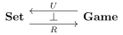
𝐒𝐞𝐭; ⟂; 𝐆𝐚𝐦𝐞; R; U

is given by R(Λ)=(ℍΛ,θΛ:ℍΛ→𝒫fin(ℍΛ))R(\Lambda)=(\mathbb{H}_{\Lambda},\theta_{\Lambda}\colon\mathbb{H}_{\Lambda}\to\mathcal{P}_{\mathrm{fin}}{(\mathbb{H}_{\Lambda})}), where the structure map θΛ\theta_{\Lambda} sends each element x=(S,λ)∈𝒫fin​(ℍΛ)×Λ=ℍΛx=(S,\lambda)\in\mathcal{P}_{\mathrm{fin}}(\mathbb{H}_{\Lambda})\times\Lambda=\mathbb{H}_{\Lambda} to θΛ​(x)=S∈𝒫fin​(ℍΛ)\theta_{\Lambda}(x)=S\in\mathcal{P}_{\mathrm{fin}}(\mathbb{H}_{\Lambda}). The counit ϵΛ:ℍΛ→Λ\epsilon_{\Lambda}\colon\mathbb{H}_{\Lambda}\to\Lambda sends each element x=(S,λ)x=(S,\lambda) to its label λ∈Λ\lambda\in\Lambda.

We will utilize this description of cofree games in the construction of the subobject classifier (Section B.5).

B.3. Some limits in 𝐆𝐚𝐦𝐞\mathbf{Game}

We have observed that the category 𝐆𝐚𝐦𝐞\mathbf{Game} has all small limits (Corollary B.10). The only example of small limits we have seen so far is the terminal object (Proposition 3.31). In this subsection, we will calculate some other finite limits.

B.3.1. Inverse image

The first example is the inverse images of subgames.

Lemma B.15.

For any game morphism f:𝕏→𝕐f\colon\mathbb{X}\to\mathbb{Y} and a subgame S⊂YS\subset Y, its inverse image f−1​(S)⊂Xf^{-1}(S)\subset X is also a subgame of 𝕏\mathbb{X}, and the diagram

f−1(S); S; 𝕏; 𝕐; f

is pullback in 𝐆𝐚𝐦𝐞\mathbf{Game}.

Proof.

One can check it directly. ∎

B.3.2. Monomorphisms

The second example of limits is monomorphisms, which is a morphism ff whose pullback along itself ff is given by two identity maps. The observations of monomorphisms in this subsubsection will be utilized to study the subobject classifier (Section B.5).

Just to avoid the following argument becoming wordy, we introduce an accessibility relation in an obvious way:

Definition B.16 (Accessibility relation).

For a game 𝕏=(X,→)\mathbb{X}=(X,\to), we say that an element x∈Xx\in X is accessible from x′x^{\prime} if there exists a non-negative integer n∈ℕn\in\mathbb{N} and a sequence of elements x0,…​xnx_{0},\dots x_{n} that satisfy

  • •

    x0=x′x_{0}=x^{\prime},

  • •

    xi→xi+1x_{i}\to x_{i+1} for 0≤i<n0\leq i<n, and

  • •

    xn=xx_{n}=x.

This accessibility relation is denoted by x′⪰xx^{\prime}\succeq x.

We write x′≻xx^{\prime}\succ x for (x′⪰x)∧(x′≠x)(x^{\prime}\succeq x)\land(x^{\prime}\neq x).

Remark B.17 (Subgames are downward closed subset).

This accessibility relation is just the reflective and transitive closure of →\to, and defines a preorder on the underlying set XX. Furthermore, due to the “finite time” condition in Definition 2.1, it is a partial order. The notion of subgames (Definition B.3) coincides with the notion of downward closed subsets of the poset.

Proposition B.18 (Subgames == Subobjects).

For any game morphism f:𝕏→𝕐f\colon\mathbb{X}\to\mathbb{Y}, the following conditions are equivalent:

  1. (1)

    ff is monic in 𝐆𝐚𝐦𝐞\mathbf{Game}.

  2. (2)

    ff is injective.

  3. (3)

    ff is (canonically isomorphic to) a subgame inclusion.

Proof.

For the equivalence between (2)(\ref{ConditionInjective}) and (3)(\ref{ConditionSubobject}), see the comment below Lemma B.4. The implication (2)⟹(1)(\ref{ConditionInjective})\implies(\ref{ConditionMonic}) immediately follows since the forgetful fucntor U:𝐆𝐚𝐦𝐞→𝐒𝐞𝐭U\colon\mathbf{Game}\to\mathbf{Set} is faithful.

We prove (1)⟹(2)(\ref{ConditionMonic})\implies(\ref{ConditionInjective}). Suppose ff is monic. We prove that #​f−1​(y)≤1\#f^{-1}(y)\leq 1 by induction on the well-founded order structure (Y,⪰)(Y,\succeq). Assuming that #​f−1​(y′)≤1\#f^{-1}(y^{\prime})\leq 1 holds for any y′≺yy^{\prime}\prec y, we prove #​f−1​(y)≤1\#f^{-1}(y)\leq 1. We can assume #​f−1​(y)≥1\#f^{-1}(y)\geq 1 since otherwise the target inequality #​f−1​(y)≤1\#f^{-1}(y)\leq 1 trivially holds. Assuming #​f−1​(y)≥1\#f^{-1}(y)\geq 1, the image of ff includes yy and hence all of y′≺yy^{\prime}\prec y (Lemma B.4), so the induction hypothesis implies

(9) #​f−1​(y′)=1​ for any ​y′≺y.\#f^{-1}(y^{\prime})=1\text{ for any }y^{\prime}\prec y.

Let us define T⊂XT\subset X as

T≔{x∈X∣f⁡(x)≺y}.T\coloneqq\{x\in X\mid f(x)\prec y\}.

Since {y′∈Y∣y′≺y}\{y^{\prime}\in Y\mid y^{\prime}\prec y\} is a subgame of 𝕐\mathbb{Y}, Lemma B.15 implies that TT is also a subgame of 𝕏\mathbb{X}. Furthermore, TT is a finite game due to Equation 9.

Adding a new element ∗\ast to TT, we extend the finite game TT into a new game 𝕎=(T∐{∗},→𝕎)\mathbb{W}=(T\coprod\{\ast\},\to_{\mathbb{W}}). In addition to the relations in TT, we add a relation ∗→𝕎t\ast\to_{\mathbb{W}}t for each t∈Tt\in T such that y→𝕐f(t)y\to_{\mathbb{Y}}f(t).

∗→𝕎t⇔y→𝕐f(t)\ast\to_{\mathbb{W}}t\iff y\to_{\mathbb{Y}}f(t)

One can prove 𝕎\mathbb{W} is actually a game, in particular satisfies the finite option condition, due to the finiteness of TT. Then, for any x∈f−1​(y)x\in f^{-1}(y), the function gx:𝕎→𝕏g_{x}\colon\mathbb{W}\to\mathbb{X} defined by

gx​(w)={t(w=t∈T)x(w=∗)g_{x}(w)=\begin{cases}t&(w=t\in T)\\ x&(w=\ast)\end{cases}

is a game morphism. It is because, for any x′∈𝕏x^{\prime}\in\mathbb{X},

x→𝕏x′\displaystyle x\to_{\mathbb{X}}x^{\prime} ⇔y=f(x)→𝕐f(x′)\displaystyle\iff y=f(x)\to_{\mathbb{Y}}f(x^{\prime})
⇔x′∈T and y→𝕐f(x′)\displaystyle\iff x^{\prime}\in T\textrm{ and }y\to_{\mathbb{Y}}f(x^{\prime})
⇔x′∈T and ∗→𝕎x′,\displaystyle\iff x^{\prime}\in T\textrm{ and }\ast\to_{\mathbb{W}}x^{\prime},

where the first inverse implication x→𝕏x′⟸f(x)→𝕐f(x′)x\to_{\mathbb{X}}x^{\prime}\impliedby f(x)\to_{\mathbb{Y}}f(x^{\prime}) holds due to the following argument: Assuming f(x)→𝕐f(x′)f(x)\to_{\mathbb{Y}}f(x^{\prime}), there exists x→𝕏x′′∈Xx\to_{\mathbb{X}}x^{\prime\prime}\in X such that f⁡(x′′)=f⁡(x′)f(x^{\prime\prime})=f(x^{\prime}) since ff satisfies the path-lifting property (Definition 3.12). Due to Equation 9, we have #​f−1​(f⁡(x′))=1\#f^{-1}(f(x^{\prime}))=1, and hence x′′=x′x^{\prime\prime}=x^{\prime}.

For any (possibly non-distinct) x0,x1∈f−1​(y)x_{0},x_{1}\in f^{-1}(y), we have a diagram

𝕎; 𝕏; 𝕐,; gx0; gx1; f

with the same composite. Since we assumed that ff is monic, we obtain gx0=gx1g_{x_{0}}=g_{x_{1}} and x0=x1x_{0}=x_{1}. This completes the proof. ∎

As UU is a faithful left adjoint, a game morphism ff is an epimorphism if and only if ff is surjective. As a corollary, the decomposition of a game morphism f:𝕏→𝕐f\colon\mathbb{X}\to\mathbb{Y} through the image game 𝕏↠Im​f↣𝕐\mathbb{X}\twoheadrightarrow\mathrm{Im}{f}\rightarrowtail\mathbb{Y} provides the epi-mono factorization system of 𝐆𝐚𝐦𝐞\mathbf{Game}.

Corollary B.19 (Epi-mono orthogonal factorization).

Any game morphism is uniquely factored into a composition of an epimorphism followed by a monomorphism. This data defines an orthogonal factorization system on 𝐆𝐚𝐦𝐞\mathbf{Game}.

Remark B.20.

In fact, this factorization system coincides with the (Epi, Regular mono) factorization system on the coregular category 𝐆𝐚𝐦𝐞\mathbf{Game}.

B.3.3. Equalizer

The third example is equalizers.

Lemma B.21 (Generation and Cogeneration of subgames).

For a game 𝕏=(X,→)\mathbb{X}=(X,\to) and a subset S⊂XS\subset X,

  • •

    there exists the minimum subgame of 𝕏\mathbb{X} that contains SS.

  • •

    there exists the maximum subgame of 𝕏\mathbb{X} that is contained by SS.

Proof.

This is an immediate corollary of the general adjoint functor theorem applied to the complete lattice inclusion from the lattice of subgames into the lattice of subsets.

Explicitly, the former subgame is constructed as

{x∈X∣∃s∈S,s⪰x},\{x\in X\mid\exists s\in S,\ s\succeq x\},

and the latter is

{x∈X∣∀y∈X,(x⪰y⟹y∈S)}\{x\in X\mid\forall y\in X,\ (x\succeq y\implies y\in S)\}

∎

The next lemma is essentially the same as [DG24, Lemma3.11].

Lemma B.22 (Equalizer in 𝐆𝐚𝐦𝐞\mathbf{Game}).

For any parallel pair of game morphisms f,g:𝕏⇉𝕐f,g\colon\mathbb{X}\rightrightarrows\mathbb{Y}, its equalizer Ef,g↣𝕏⇉𝕐E_{f,g}\rightarrowtail\mathbb{X}\rightrightarrows\mathbb{Y} is given by

Ef,g={x∈X∣∀x′⪯x,f(x′)=g(x′)}.E_{f,g}=\{x\in X\mid\forall x^{\prime}\preceq x,f(x^{\prime})=g(x^{\prime})\}.
Proof.

For any game morphism h:𝕎→𝕏h\colon\mathbb{W}\to\mathbb{X} such that f∘h=g∘hf\circ h=g\circ h, the image Im​h\mathrm{Im}{h} is a subgame contained by the set-theoretic equalizer E0={x∈X∣f⁡(x)=g⁡(x)}E_{0}=\{x\in X\mid f(x)=g(x)\}. Since Ef,gE_{f,g} is the maximum subgame contained by E0E_{0} in the sense of Lemma B.21, we have Im​h⊂Ef,g\mathrm{Im}{h}\subset E_{f,g}, and hh factors through the subgame inclusion Ef,g↣𝕏E_{f,g}\rightarrowtail\mathbb{X}. The uniqueness part of the universality trivially holds since Ef,g↣𝕏E_{f,g}\rightarrowtail\mathbb{X} is injective. ∎

B.3.4. Digression: General limits and Stirling numbers

As UU is not continuous, it is not easy to calculate genral limits in 𝐆𝐚𝐦𝐞\mathbf{Game}. However, there is a (non-efficient) way to calculate limits using the cofree games functor (Section B.2): Take an arbitrary small diagram F:J→𝐆𝐚𝐦𝐞F\colon J\to\mathbf{Game}. Due to Corollary B.10, we know that limF\lim F exists. So we have

𝐆𝐚𝐦𝐞⁡(𝕏,limF)≅\displaystyle\mathbf{Game}(\mathbb{X},\lim F)\cong 𝐂𝐨𝐧𝐞𝐆𝐚𝐦𝐞​(𝕏,F)\displaystyle\mathbf{Cone}_{\mathbf{Game}}(\mathbb{X},F)
⊂\displaystyle\subset 𝐂𝐨𝐧𝐞𝐒𝐞𝐭​(U​𝕏,U​F)\displaystyle\mathbf{Cone}_{\mathbf{Set}}(U\mathbb{X},UF)
≅\displaystyle\cong 𝐒𝐞𝐭⁡(U​𝕏,limU​F)\displaystyle\mathbf{Set}(U\mathbb{X},\lim UF)
≅\displaystyle\cong 𝐆𝐚𝐦𝐞⁡(𝕏,R​limU​F),\displaystyle\mathbf{Game}(\mathbb{X},R\lim UF),

where RR denotes the cofree game functor, which is the right adjoint to UU (Proposition B.14). Therefore, we conclude that limF\lim F is a subgame of R​limU​FR\lim UF, whose underlying set is given by the limU​F\lim UF-labeled hereditarily finite set ℍlimU​F\mathbb{H}_{\lim UF}. As this observation works for any faithful left adjoint functor UU, it loses a lot of information and it is not always easy to figure out which subgame is the limit.

Let us demonstrate how general limits are difficult to calculate. For a positive integer n>0n>0, let 𝕊n\mathbb{S}_{n} denote the (n+1)(n+1)-state game that looks like Figure 15.

Diagram
Figure 15. The game 𝕊n\mathbb{S}_{n} for n=5n=5

Then, the product game 𝕊2×𝕊3\mathbb{S}_{2}\times\mathbb{S}_{3} looks like Figure 16.

Diagram
Figure 16. The pruduct game 𝕊2×𝕊3\mathbb{S}_{2}\times\mathbb{S}_{3}, which categorifies
2!​S​(n,2)×3!​S​(n,3)=1⋅6!​S​(n,6)+6⋅5!​S​(n,5)+12⋅4!​S​(n,4)+6⋅3!​S​(n,3)2!S(n,2)\times 3!S(n,3)=1\cdot 6!S(n,6)+6\cdot 5!S(n,5)+12\cdot 4!S(n,4)+6\cdot 3!S(n,3).

What is happning there? One interpretation is given by regarding 𝕊k\mathbb{S}_{k} as an categorification of the Stirling number of the second kind!

One can easily prove that #​𝐆𝐚𝐦𝐞​(𝕊n,𝕊k)\#\mathbf{Game}(\mathbb{S}_{n},\mathbb{S}_{k}) is the number of surjections from an nn-element set to an mm-element set, which is known to be equal to k!​S​(n,k)k!S(n,k), where S⁡(n,k)S(n,k) is the Stirling number of the second kind.

#​𝐆𝐚𝐦𝐞​(𝕊n,𝕊k)=k!​S​(n,k)\#\mathbf{Game}(\mathbb{S}_{n},\mathbb{S}_{k})=k!S(n,k)

Therefore, the product game 𝕊2×𝕊3\mathbb{S}_{2}\times\mathbb{S}_{3} should have information about 2!​S​(n,2)×3!​S​(n,3)2!S(n,2)\times 3!S(n,3) since the following equality holds.

𝐆𝐚𝐦𝐞⁡(𝕊n,𝕊2×𝕊3)≅𝐆𝐚𝐦𝐞⁡(𝕊n,𝕊2)×𝐆𝐚𝐦𝐞⁡(𝕊n,𝕊3)\mathbf{Game}(\mathbb{S}_{n},\mathbb{S}_{2}\times\mathbb{S}_{3})\cong\mathbf{Game}(\mathbb{S}_{n},\mathbb{S}_{2})\times\mathbf{Game}(\mathbb{S}_{n},\mathbb{S}_{3})

In fact, the product game (or, more precisely, the isomorphism to its concrete description Figure 16) is a categorification of the multiplicative identity of the Stirling number:

2!​S​(n,2)×3!​S​(n,3)=1⋅6!​S​(n,6)+6⋅5!​S​(n,5)+12⋅4!​S​(n,4)+6⋅3!​S​(n,3).2!S(n,2)\times 3!S(n,3)=1\cdot 6!S(n,6)+6\cdot 5!S(n,5)+12\cdot 4!S(n,4)+6\cdot 3!S(n,3).

Notice that these coefficients 1,6,12,61,6,12,6 appear in Figure 16.

Even the inocent-looking example 𝕊n×𝕊m\mathbb{S}_{n}\times\mathbb{S}_{m} is interwinded with the combinatorics of the Stirling numbers. By this example, we would like to emphasize the difficulty of the calculation of general limits in 𝐆𝐚𝐦𝐞\mathbf{Game}.

B.4. 𝐆𝐚𝐦𝐞\mathbf{Game} is comonadic over 𝐒𝐞𝐭\mathbf{Set}

The following proof is essentially the same as the comonadicity of locally finite Kriple frames [DG24, Theorem 5.4].

Proposition B.23.

The forgetful functor U:𝐆𝐚𝐦𝐞→𝐒𝐞𝐭U\colon\mathbf{Game}\to\mathbf{Set} is comonadic.

Proof.

We use the reflexive tripleability theorem (see [Rie17, Propotition 5.5.8]). As we have already proven that UU is a consevative left adjoint functor (Lemma B.2 and Corollary B.12) and 𝐆𝐚𝐦𝐞\mathbf{Game} is complete (Corollary B.10), it suffices to prove that UU preserves equalizers of coreflexive pairs.

Take an arbitrary coreflexive pair f,g:𝕏⇉𝕐f,g\colon\mathbb{X}\rightrightarrows\mathbb{Y} with a common retract r:𝕐→𝕏r\colon\mathbb{Y}\to\mathbb{X} such that r∘f=r∘g=id𝕏r\circ f=r\circ g=\mathrm{id}_{\mathbb{X}}. Then, due to Lemma B.22, the equalizer is given by Ef,g={x∈X∣∀x′⪯x,f(x′)=g(x′)}E_{f,g}=\{x\in X\mid\forall x^{\prime}\preceq x,\;f(x^{\prime})=g(x^{\prime})\}. We should prove that this coincides with the set-theoretic equalizer {x∈X∣f⁡(x)=g⁡(x)}\{x\in X\mid f(x)=g(x)\}.

Therefore, it suffices to prove that, for any x→𝕏x′x\to_{\mathbb{X}}x^{\prime}, f⁡(x)=g⁡(x)f(x)=g(x) implies f⁡(x′)=g⁡(x′)f(x^{\prime})=g(x^{\prime}). Assuming f⁡(x)=g⁡(x)f(x)=g(x) and x→𝕏x′x\to_{\mathbb{X}}x^{\prime}, we can take x→𝕏x′′x\to_{\mathbb{X}}x^{\prime\prime} such that f⁡(x′′)=g⁡(x′)f(x^{\prime\prime})=g(x^{\prime}) by applying the path-lifting property to f(x)=g(x)→𝕐g(x′)f(x)=g(x)\to_{\mathbb{Y}}g(x^{\prime}). By applying the common retract rr to the equation f⁡(x′′)=g⁡(x′)f(x^{\prime\prime})=g(x^{\prime}), we obtain x′′=x′x^{\prime\prime}=x^{\prime}, which implies f⁡(x′)=f⁡(x′′)=g⁡(x′)f(x^{\prime})=f(x^{\prime\prime})=g(x^{\prime}). This completes the proof. ∎

B.5. 𝐆𝐚𝐦𝐞\mathbf{Game} has a subobject classifier

In this subsection, we will give an explicit description of the subobject classifier of the category of games.

Our idea of the construction is simple: utilize the cofree-forgetful adjunction (Proposition B.14). As subobjects are just subsets satisfying some properties (Proposition B.18), we have the following canonical injection

(10) Sub𝐆𝐚𝐦𝐞​(𝕏)⊂𝒫⁡(X)≅𝐒𝐞𝐭⁡(X,{⊤,⊥})≅𝐆𝐚𝐦𝐞⁡(𝕏,ℍ{⊤,⊥}).\mathrm{Sub}_{\mathbf{Game}}(\mathbb{X})\subset\mathcal{P}(X)\cong\mathbf{Set}(X,\{\top,\bot\})\cong\mathbf{Game}(\mathbb{X},\mathbb{H}_{\{\top,\bot\}}).

Therefore, by the Yoneda lemma, if a subobject classifier Ω\Omega exists, then it should be a subobject of the game of truth-values-labeled hereditarily finite sets Ω⊂ℍ{⊤,⊥}\Omega\subset\mathbb{H}_{\{\top,\bot\}}.

Let us recall how the correspondence 𝒫⁡(X)≅𝐒𝐞𝐭⁡(X,{⊤,⊥})≅𝐆𝐚𝐦𝐞⁡(𝕏,ℍ{⊤,⊥})\mathcal{P}(X)\cong\mathbf{Set}(X,\{\top,\bot\})\cong\mathbf{Game}(\mathbb{X},\mathbb{H}_{\{\top,\bot\}}) in (10) works. Let 𝕏=(X,θ)\mathbb{X}=(X,\theta) be a game and S⊂XS\subset X be a subset. Then, the corresponding game morphism χS:𝕏→ℍ{⊤,⊥}\chi_{S}\colon\mathbb{X}\to\mathbb{H}_{\{\top,\bot\}} sends an element x∈Xx\in X to

χS(x)=({χS(x′)∣x→𝕏x′},x∈S)∈𝒫fin(ℍ{⊤,⊥})×{⊤,⊥}=ℍ{⊤,⊥},\chi_{S}(x)=\left(\{\chi_{S}(x^{\prime})\mid x\to_{\mathbb{X}}x^{\prime}\},x\in S\right)\in\mathcal{P}_{\mathrm{fin}}\left(\mathbb{H}_{\{\top,\bot\}}\right)\times\{\top,\bot\}=\mathbb{H}_{\{\top,\bot\}},

where “x∈Sx\in S” denotes the element of {⊤,⊥}\{\top,\bot\} corresponding to the truth value of the proposition “x∈Sx\in S.” Conversely, for a given game morphism f:𝕏→ℍ{⊤,⊥}f\colon\mathbb{X}\to\mathbb{H}_{\{\top,\bot\}}, the corresponding subset is recovered by taking {x∈X∣the label of f⁡(x) is ⊤}\{x\in X\mid\text{the label of $f(x)$ is $\top$}\}. An example of such χS\chi_{S} (in the case where SS is a subgame of 𝕏\mathbb{X}) is visualized in Figure 17, where ⊤{\color[rgb]{1,0,0}\top} and ⊥\bot are colored like (8).

{{{{}}}{{{}}{{}{}}}}; {{{}}{{}{}}}; {{}{}}; {}; {{{}}}; {{}}; {}; {}; {{}}; {}; {}
Figure 17. The characteristic map χS\chi_{S} for a subgame SS
Definition B.24.

A {⊤,⊥}\{\top,\bot\}-labeled hereditarily finite set A∈ℍ{⊤,⊥}A\in\mathbb{H}_{\{\top,\bot\}} is truth-closed if

  1. (1)

    if AA itself is labeled by ⊤\top, then every element of AA is also labeled by ⊤\top, and

  2. (2)

    every element of AA is truth-closed.

Due to condition (2), truth-closed {⊤,⊥}\{\top,\bot\}-labeled hereditarily finite sets form a subgame of ℍ{⊤,⊥}\mathbb{H}_{\{\top,\bot\}}. By coloring like (8), the typical examples of a truth-closed {⊤,⊥}\{{\color[rgb]{1,0,0}\top},\bot\}-labeled set include {}{\color[rgb]{1,0,0}\{\}}, {}{\color[rgb]{0,0,0}\{\}}, {{{{{}}}}}{\color[rgb]{0,0,0}\{{\color[rgb]{0,0,0}\{{\color[rgb]{0,0,0}\{{\color[rgb]{1,0,0}\{{\color[rgb]{1,0,0}\{\}}\}}\}}\}}\}}, and {{{{}}}​{{}​{{}}}​{{}}}{\color[rgb]{0,0,0}\{{\color[rgb]{0,0,0}\{{\color[rgb]{0,0,0}\{{\color[rgb]{1,0,0}\{\}}\}}\}}{\color[rgb]{1,0,0}\{{\color[rgb]{1,0,0}\{\}}{\color[rgb]{1,0,0}\{{\color[rgb]{1,0,0}\{\}}\}}\}}{\color[rgb]{0,0,0}\{{\color[rgb]{0,0,0}\{\}}\}}\}}. Non-examples include {{}}{\color[rgb]{1,0,0}\{{\color[rgb]{0,0,0}\{\}}\}} and {{}​{{{}}}}{\color[rgb]{0,0,0}\{{\color[rgb]{0,0,0}\{\}}{\color[rgb]{1,0,0}\{{\color[rgb]{0,0,0}\{{\color[rgb]{1,0,0}\{\}}\}}\}}\}}. Intuitively, a {⊤,⊥}\{{\color[rgb]{1,0,0}\top},\bot\}-labeled hereditarily finite set is truth-closed if and only if no black parenthesis appears within any red parenthesis.

Notation B.25.

The subgame of ℍ{⊤,⊥}\mathbb{H}_{\{\top,\bot\}} consisting of all truth-closed {⊤,⊥}\{\top,\bot\}-labeled hereditarily finite sets is denoted by Ω\Omega.

The game Ω\Omega is visualized in Figure 18.

{}; {}; {{}}; {{}}; {{}{}}; {{}}; {{{}}}; {{{}}}; {{{}{}}}; {{{}}}; {{{}}}; {{}{{}}}; {{}{{}}}; {{}{{}{}}}; {{}{}}; {{}{{}}}; {{{}}{{}}}; {{{}}{{}{}}}; {{}{{}}}; {{{}}{}}; {{{}}{{}}}; {{{}}{{}{}}}; {{{}}{}}; {{{}}{{}}}; {{{}{}}{}}; {{{}{}}{{}}}; {{}{{}}}; ⋮
Figure 18. A partial sketch of the subobject classifier Ω\Omega
Proposition B.26 (Subobject classifier).

The game Ω\Omega is the subobject classifier of the category of games 𝐆𝐚𝐦𝐞\mathbf{Game}.

Proof.

We prove that, for any subset S⊂XS\subset X of any game 𝕏=(X,θ)\mathbb{X}=(X,\theta), SS is a subgame if and only if the characteristic map χS:𝕏→ℍ{⊤,⊥}\chi_{S}\colon\mathbb{X}\to\mathbb{H}_{\{\top,\bot\}} factors through the subgame Ω↣ℍ{⊤,⊥}\Omega\rightarrowtail\mathbb{H}_{\{\top,\bot\}}.

Assuming that SS is a subgame, we prove that χS​(x)\chi_{S}(x) is truth-closed for any x∈Xx\in X by induction. At the step of x∈Xx\in X, the condition (2) in Definition B.24 is verified by the induction hypothesis. Regarding condition (1), if χS​(x)\chi_{S}(x) is labeled by ⊤\top, i.e., x∈Sx\in S, then every χS​(x′)\chi_{S}(x^{\prime}) is also labeled by ⊤\top for any x→𝕏x′x\to_{\mathbb{X}}x^{\prime}, since SS is a subgame.

Conversely, assume that χS\chi_{S} factors through Ω\Omega. Then, for any x∈Sx\in S, χS​(x)\chi_{S}(x) is truth-closed and labeled by ⊤\top. Therefore, for every x→𝕏x′x\to_{\mathbb{X}}x^{\prime}, χS​(x′)\chi_{S}(x^{\prime}) is also labeled by ⊤\top, which implies that SS is a subgame. ∎

Remark B.27 (𝐆𝐚𝐦𝐞\mathbf{Game} is not a topos).

The reader may wonder if 𝐆𝐚𝐦𝐞\mathbf{Game} is a Grothendieck topos, since it satisfies a lot of nice properties like topos, including the existence of a subobject classifier, epi-mono factorization system, the frame structure of the subobject lattice, local finite presentability, and so on. Unfortunately, 𝐆𝐚𝐦𝐞\mathbf{Game} is not even cartesian closed. In fact, the product functor 𝕊2×−:𝐆𝐚𝐦𝐞→𝐆𝐚𝐦𝐞\mathbb{S}_{2}\times{-}\colon\mathbf{Game}\to\mathbf{Game} does not preserve colimits (cf. Figure 15). For example, the colimit of the canonical ℤ/2​ℤ\mathbb{Z}/2\mathbb{Z}-action on 𝕊2\mathbb{S}_{2} is 𝕊1\mathbb{S}_{1}. However, the colimit of induced ℤ/2​ℤ\mathbb{Z}/2\mathbb{Z}-action on 𝕊2×𝕊2\mathbb{S}_{2}\times\mathbb{S}_{2} has 66 elements.

colimℤ/2​ℤ(𝕊2×𝕊2)→non-iso𝕊2×colimℤ/2​ℤ𝕊2=𝕊2×𝕊1=𝕊2\colim_{\mathbb{Z}/2\mathbb{Z}}\left(\mathbb{S}_{2}\times\mathbb{S}_{2}\right)\xrightarrow{\text{non-iso}}\mathbb{S}_{2}\times\colim_{\mathbb{Z}/2\mathbb{Z}}\mathbb{S}_{2}=\mathbb{S}_{2}\times\mathbb{S}_{1}=\mathbb{S}_{2}

This shows that the functor 𝕊2×−\mathbb{S}_{2}\times{-} is not cocontinuous; in particular, 𝐆𝐚𝐦𝐞\mathbf{Game} is neither cartesian closed nor a topos.

Appendix C Birthday ⊣\dashv Nim ⊣\dashv Grundy number

The Bouton theorem (Theorem 2.9) looks particularly simple due to the fact that the Grundy number map 𝖦𝗋𝗎𝗇𝖽𝗒Nim1:ℕ→ℕ\mathsf{Grundy}_{\mathrm{Nim}_{1}}\colon\mathbb{N}\to\mathbb{N} turns out to be the identity map idℕ\mathrm{id}_{\mathbb{N}} (cf. Example 2.18). The aim of this appendix is to explain this coincidence 𝖦𝗋𝗎𝗇𝖽𝗒Nim1=idℕ\mathsf{Grundy}_{\mathrm{Nim}_{1}}=\mathrm{id}_{\mathbb{N}} by a “categorical origin” of the mex function 𝗆𝖾𝗑:𝒫fin​(ℕ)→ℕ\mathsf{mex}\colon\mathcal{P}_{\mathrm{fin}}(\mathbb{N})\to\mathbb{N}.

We start with a simple observation.

Proposition C.1.

For an endofunctor T:𝒞→𝒞T\colon\mathcal{C}\to\mathcal{C} on a category 𝒞\mathcal{C}, a TT-algebra 𝔸=(A,α)\mathbb{A}=(A,\alpha), and a recursive TT-coalgebra 𝕏=(A,θ)\mathbb{X}=(A,\theta) on the same object A∈ob⁡(𝒞)A\in\mathrm{ob}(\mathcal{C}), the following two condtions are equivalent.

  1. (1)

    θ\theta is the section of α\alpha, i.e., α∘θ=idA\alpha\circ\theta=\mathrm{id}_{A}.

  2. (2)

    The hylomorphism 𝗁𝗒𝗅𝗈𝔸,𝕏:A→A\mathsf{hylo}_{\mathbb{A},\mathbb{X}}\colon A\to A coincides with the identity map idA\mathrm{id}_{A}.

Proof.

Both conditions are equivalent to the commutativity of

TA; TA; A; A.; T⁡(idA); α; θ; idA

∎

Therefore, unsurprisingly, the coincidence 𝖦𝗋𝗎𝗇𝖽𝗒Nim1(=𝗁𝗒𝗅𝗈𝖬𝖾𝗑,Nim1)=idℕ\mathsf{Grundy}_{\mathrm{Nim}_{1}}(=\mathsf{hylo}_{\mathsf{Mex},\mathrm{Nim}_{1}})=\mathrm{id}_{\mathbb{N}} comes from the fact that the structure map of nim ν\nu is a section of 𝗆𝖾𝗑\mathsf{mex}, i.e., 𝗆𝖾𝗑∘ν=idℕ\mathsf{mex}\circ\nu=\mathrm{id}_{\mathbb{N}}

𝗆𝖾𝗑∘ν⁡(n)=𝗆𝖾𝗑⁡{0,1,…,n−1}=n.\mathsf{mex}\circ\nu(n)=\mathsf{mex}\{0,1,\dots,n-1\}=n.

What might be a bit surprising is that 𝗆𝖾𝗑\mathsf{mex} is actually the canonical choice of a retraction of ν\nu in a categorical sence! When a canonical “reverse” of a map ν:ℕ→𝒫fin​(ℕ)\nu\colon\mathbb{N}\to\mathcal{P}_{\mathrm{fin}}(\mathbb{N}) is needed, we category theorists think like “ok, then consider its adjoint!”
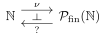
ℕ; 𝒫fin(ℕ); ν; ?; ⊣

And the adjoint turns out to be mex! Here, we consider the usual order on each set, namely, the usual order ≤\leq on ℕ\mathbb{N} and the inclusion relation on 𝒫fin​(ℕ)\mathcal{P}_{\mathrm{fin}}(\mathbb{N}).

Proposition C.2 (A characterization of mex).

The right adjoint of ν\nu is 𝗆𝖾𝗑\mathsf{mex}.

ℕ; 𝒫fin(ℕ); ν; 𝗆𝖾𝗑; ⊣
Proof.

Take any n∈ℕn\in\mathbb{N} and S∈𝒫fin​(ℕ)S\in\mathcal{P}_{\mathrm{fin}}(\mathbb{N}). Then, we have

n≤𝗆𝖾𝗑​S\displaystyle n\leq\mathsf{mex}{S} ⇔n≤min⁡Sc\displaystyle\iff n\leq\min{S^{\mathrm{c}}}
⇔ν​(n)c⊃Sc\displaystyle\iff\nu(n)^{\mathrm{c}}\supset S^{\mathrm{c}}
⇔ν⁡(n)⊂S.\displaystyle\iff\nu(n)\subset S.

∎

Since ν\nu is fully faithful, its right adjoint 𝗆𝖾𝗑\mathsf{mex} should be a retract of ν\nu thanks to the general theory of adjoint functors (and the skeletality of the posets). So we can apply Proposition C.1.

Similar phenomena are ubiquitous in this paper. For example, ν:ℕ→𝒫fin​(ℕ)\nu\colon\mathbb{N}\to\mathcal{P}_{\mathrm{fin}}(\mathbb{N}) also admits a right adjoint, which turns out to be 𝗑𝖾𝗆\mathsf{xem}!

ℕ; 𝒫fin(ℕ); ν; 𝗑𝖾𝗆; ⊣

Therefore, Proposition C.1 implies that 𝖡𝗂𝗋𝗍𝗁𝖣𝖺𝗒Nim1:ℕ→ℕ\mathsf{BirthDay}_{\mathrm{Nim}_{1}}\colon\mathbb{N}\to\mathbb{N} is also the identity map. This is the meaning of the title of this appendix: Birthday ⊣\dashv Nim ⊣\dashv Grundy number, which actually means

𝗑𝖾𝗆⊣ν⊣𝗆𝖾𝗑.\mathsf{xem}\dashv\nu\dashv\mathsf{mex}.

Another example is the remoteness.

Example C.3.

The game ElM\mathrm{ElM} (Example 2.7) is a section of the remoteness (Example 3.24) up to a canonical bijection.

References

  • [Ack37] Wilhelm Ackermann “Die widerspruchsfreiheit der allgemeinen mengenlehre” In Mathematische Annalen 114.1 Springer, 1937, pp. 305–315
  • [Adá74] Jiří Adámek “Free algebras and automata realizations in the language of categories” In Commentationes Mathematicae Universitatis Carolinae 15.4 Charles University in Prague, Faculty of MathematicsPhysics, 1974, pp. 589–602
  • [Adá05] Jiří Adámek “Introduction to coalgebra” In Theory and Applications of Categories 14.8, 2005, pp. 157–199
  • [ALM07] Jiří Adámek, Dominik Lücke and Stefan Milius “Recursive coalgebras of finitary functors” In RAIRO-Theoretical Informatics and Applications 41.4 EDP Sciences, 2007, pp. 447–462
  • [AMM20] Jiří Adámek, Stefan Milius and Lawrence Moss “On Well-Founded and Recursive Coalgebras.” In FoSSaCS, 2020, pp. 17–36
  • [AR94] Jiří Adámek and Jiří Rosickỳ “Locally Presentable and Accessible Categories” Cambridge University Press, 1994
  • [BS09] John. Baez and Michael Shulman “Lectures on n-categories and cohomology” In Towards higher categories Springer, 2009, pp. 1–68
  • [BES25] Mikhail Baltushkin, Dana. Ernst and Nándor Sieben “Isomorphism Theorems for Impartial Combinatorial Games” In arXiv preprint arXiv:2505.04919, 2025
  • [Baš+24] Bojan Bašić et al. “Categories of impartial rulegraphs and gamegraphs” In International Journal of Game Theory Springer, 2024, pp. 1–27
  • [Bou01] Charles. Bouton “Nim, a game with a complete mathematical theory” In Annals of mathematics 3.1/4 JSTOR, 1901, pp. 35–39
  • [BS81] Stanley Burris and H.. Sankappanavar “A course in universal algebra” 78, Graduate Texts in Mathematics Springer-Verlag, New York-Berlin, 1981, pp. xvi+276
  • [CUV06] Venanzio Capretta, Tarmo Uustalu and Varmo Vene “Recursive coalgebras from comonads” In Information and Computation 204.4 Elsevier, 2006, pp. 437–468
  • [CP20] Thomas Colcombet and Daniela Petrişan “Automata minimization: a functorial approach” In Logical Methods in Computer Science 16 Episciences. org, 2020
  • [Con00] John. Conway “On numbers and games” AK Peters/CRC Press, 2000
  • [DG24] Matteo De and Silvio Ghilardi “Profiniteness, monadicity and universal models in modal logic” In Annals of Pure and Applied Logic 175.7 Elsevier, 2024, pp. 103454
  • [DH13] Matthieu Dufour and Silvia Heubach “Circular Nim Games” In the electronic journal of combinatorics 20.2, 2013, pp. P22
  • [FLK80] François Foltz, Christian Lair and Gregory. Kelly “Algebraic categories with few monoidal biclosed structures or none” In Journal of Pure and Applied Algebra 17.2 North-Holland, 1980, pp. 171–177
  • [HL09] Furio Honsell and Marina Lenisa “Conway games, coalgebraically” In Algebra and Coalgebra in Computer Science: Third International Conference, CALCO 2009, Udine, Italy, September 7-10, 2009. Proceedings 3, 2009, pp. 300–316 Springer
  • [Jac16] Bart Jacobs “Bisimulations” In Introduction to Coalgebra: Towards Mathematics of States and Observation, Cambridge Tracts in Theoretical Computer Science Cambridge University Press, 2016, pp. 114–158
  • [Jac17] Bart Jacobs “Introduction to coalgebra” Cambridge University Press, 2017
  • [Joy77] André Joyal “Remarques sur la théorie des jeux à deux personnes” In Gazette des sciences mathématiques du Québec 1.4, 1977, pp. 46–52
  • [KK24] Krzysztof Kapulkin and Nathan Kershaw “Closed symmetric monoidal structures on the category of graphs” In Theory and Applications of Categories 41.23, 2024, pp. 760–784
  • [Kun13] Kenneth Kunen “Set Theory” 34, Studies in logic College Publications, 2013
  • [Lam68] Joachim Lambek “A fixpoint theorem for complete categories” In Mathematische Zeitschrift 103.2 Springer, 1968, pp. 151–161
  • [Mac98] Saunders Mac “Categories for the working mathematician”, Graduate Texts in Mathematics Springer-Verlag, New York, 1998, pp. xii+314
  • [Osi74] Gerhard Osius “Categorical set theory: a characterization of the category of sets” In Journal of Pure and Applied Algebra 4.1 Elsevier, 1974, pp. 79–119
  • [Pin22] Jean-Éric Pin “Mathematical foundations of automata theory”, 2022
  • [Poh73] Věra Pohlová “On sums in generalized algebraic categories” In Czechoslovak Mathematical Journal 23.2 Institute of Mathematics, Academy of Sciences of the Czech Republic, 1973, pp. 235–251
  • [Rie17] Emily Riehl “Category theory in context” Courier Dover Publications, 2017
  • [Sie13] Aaron. Siegel “Combinatorial game theory” American Mathematical Soc., 2013
  • [Smi66] Cedric.B. Smith “Graphs and composite games” In Journal of Combinatorial Theory 1.1 Academic Press, 1966, pp. 51–81
  • [Tay99] Paul Taylor “Practical foundations of mathematics” Cambridge University Press, 1999

Internal hom for Conway addition§

Question and proposed construction

Question 5.7 of Games as recursive coalgebras asks for a concrete right adjoint to Conway addition:

Game(G+K,H)≅Game(K,[G,H]+). \mathbf{Game}(G+K,H)\cong\mathbf{Game}(K,[G,H]_+).

Existence is proved abstractly in the paper. The proposed construction and proof below describe positions, moves, evaluation, and currying explicitly. A detailed proposed proof is in note 29.

Positions and moves

Put S=Set⁡(UG,UH)S=\operatorname{Set}(UG,UH). By Definition B.13 and Proposition B.14, the cofree game R(S)R(S) consists of hereditarily finite labelled positions t=(Tt,at)t=(T_t,a_t), with finite child set TtT_t and label at∈Sa_t\in S.

Let A(G,H)A(G,H) consist of those t∈R(S)t\in R(S) for which every descendant ww, including tt, satisfies

θH(aw(g))={aw(g′):g′∈θG(g)}∪{av(g):v∈Tw}(g∈UG). \theta_H(a_w(g)) =\{a_w(g'):g'\in\theta_G(g)\} \cup\{a_v(g):v\in T_w\} \quad(g\in UG).

The condition is inherited by children, so A(G,H)A(G,H) is a subgame. Its moves are the inherited child relation.

Evaluation and currying

Evaluation is ev⁡(g,t)=at(g)\operatorname{ev}(g,t)=a_t(g). The displayed equation says exactly that it is an exact coalgebra morphism G+A(G,H)→HG+A(G,H)\to H.

For a morphism f:G+K→Hf:G+K\to H, take the cofree transpose of the label map k↦(g↦f(g,k))k\mapsto(g\mapsto f(g,k)):

hf(k)=({hf(k′):k′∈θK(k)}, g↦f(g,k)). h_f(k)=\bigl(\{h_f(k'):k'\in\theta_K(k)\},\,g\mapsto f(g,k)\bigr).

The morphism equation for ff gives the compatibility equation at every image position. The image is closed under options, so hfh_f factors through A(G,H)A(G,H). Conversely, evaluation uncurries any map K→A(G,H)K\to A(G,H). One composite is the identity by evaluation of labels; the other is the identity by uniqueness of the cofree transpose. Thus A(G,H)A(G,H) is the required right adjoint.

This is a construction in the category of finitely branching, finite-time games with exact coalgebra maps. The carriers need not be finite.

Status and remaining work

This is a proposed construction and proof, retained as a proof candidate rather than a human-reviewed result. The argument is stated in the precise category stated above; it does not claim a new published theorem or a completed human review.

Compute usable small examples and explain the game-theoretic meaning of these labelled positions. The construction does not identify this internal hom with player-switching or a strategy-category internal hom. It does not establish the partisan analogue. Its relation to prior mapping-object constructions also requires a separate literature comparison.

Exact completion of games and the Leibniz obstruction§

○ AI-claimed○ Human-claimed○ LEAN formalized

Current result and proof status

The category of games is not itself a topos; see the original question. The proposed replacement is its exact completion, presented as sheaves on finite games. This note records that construction and a concrete obstruction to its proposed differential structure: the Leibniz law below gives 6 maps on one side and 2 on the other.

The exact-completion and Day-tensor arguments are in the linked manuscripts. The finite map counts below are explicit; their interpretation as a sheaf counterexample uses the embedding and closed-tensor results. The open questions below remain separate from those results.

Definitions and the exact-completion construction

Let Games=RecCoalg⁡(Pf)\mathrm{Games}=\operatorname{RecCoalg}(P_f), with maps satisfying
succ⁡(f(x))=f[succ⁡(x)]\operatorname{succ}(f(x))=f[\operatorname{succ}(x)].
Let Gamesfin\mathrm{Games}_{\mathrm{fin}} be the full subcategory on finite carriers, and let JcohJ_{\mathrm{coh}} be generated by finite jointly surjective families. Put

E=Sh⁡(Gamesfin,Jcoh),N(X)=Games(−,X)∣Gamesfin. \mathcal E=\operatorname{Sh}(\mathrm{Games}_{\mathrm{fin}},J_{\mathrm{coh}}), \qquad N(X)=\mathrm{Games}(-,X)|_{\mathrm{Games}_{\mathrm{fin}}}.

Write Starm\mathrm{Star}_m for a root with mm terminal children.

The construction asserts that Games is regular, with epimorphisms equal to surjections and regular epimorphisms, stable under pullback. It is infinitary extensive but not exact: Δ∪Γσ⊆Star2×Star2\Delta\cup\Gamma_\sigma\subseteq\mathrm{Star}_2\times\mathrm{Star}_2, with σ\sigma swapping the two terminal children, is a six-element noneffective equivalence relation. Its ex/reg completion is

Map⁡(Games)≃E. \operatorname{Map}(\mathrm{Games})\simeq\mathcal E.

The proof uses that every subobject of N(X)N(X) comes from a subgame and that NN preserves coproducts, surjections, and filtered colimits. The subobject classifier is ΩE=N(ΩGames)\Omega_{\mathcal E}=N(\Omega_{\mathrm{Games}}), described using truth-closed hereditarily finite sets.

An exact-completion object (X,R)(X,R) retains a game together with witnesses of its equivalence relation. A quotient is already represented in Games when its relation is a kernel pair. In particular,
Q=N(Star2)/(Δ∪Γσ)Q=N(\mathrm{Star}_2)/(\Delta\cup\Gamma_\sigma)
is outside the image of NN; it has N(Star1)N(\mathrm{Star}_1) as a quotient, not as a claimed retract.

Properties asserted by the construction

  • The terminal object is N(V)N(V), where VV is the game of all hereditarily finite sets. It is not quasi-compact, so E\mathcal E is not coherent. The subterminal objects N(V<n)N(V_{<n}) give an open cover by coherent topoi
    En≃Sh⁡((Gamesfin)<n,Jcoh)\mathcal E_n\simeq\operatorname{Sh}((\mathrm{Games}_{\mathrm{fin}})_{<n},J_{\mathrm{coh}}).
    Thus E\mathcal E has enough points. Its proposed geometric theory combines the coherent theories at each finite height with the infinitary assertion that every position has some finite height.
  • E1≃Set\mathcal E_1\simeq\mathrm{Set} is a dense open point and Sh⁡¬¬(E)≃Set\operatorname{Sh}_{\neg\neg}(\mathcal E)\simeq\mathrm{Set}. The point is given by the terminal-position functor. The one-position no-move game is projective; so is every finite discrete no-move game. No uniqueness or classification of connected projectives is claimed here.
  • E\mathcal E is not Boolean: the terminal-position subgame of Star1\mathrm{Star}_1 has no complement. It is not localic: N(Star2)N(\mathrm{Star}_2) is not covered by subterminal objects. Its proposed localic reflection is the presheaf topos on (Vω,∈+)(V_\omega,\in^+).
  • A proposed family of points, indexed by nonempty perfect Stone spaces SS, is
    FS(X)={(x,e):succ⁡(x) consists of terminal positions, e:S↠succ⁡(x) continuous}F_S(X)=\{(x,e):\operatorname{succ}(x)\text{ consists of terminal positions},\ e:S\twoheadrightarrow\operatorname{succ}(x)\text{ continuous}\}.
    This is not a classification of all points.

Conway addition and the tensor

Conway addition ++ is not left exact: the comparison involving
(Star2×Star1Star2)+Star1(\mathrm{Star}_2\times_{\mathrm{Star}_1}\mathrm{Star}_2)+\mathrm{Star}_1
and
(Star2+Star1)×Star1+Star1(Star2+Star1)(\mathrm{Star}_2+\mathrm{Star}_1)\times_{\mathrm{Star}_1+\mathrm{Star}_1}(\mathrm{Star}_2+\mathrm{Star}_1)
has respectively 77 and 7⋅1277\cdot127 roots. Therefore its descent to the completion cannot simply use the 2-functoriality of ex/reg completion on left-exact functors.

The proposed alternative is the sheafified Day tensor ⊕\oplus on E\mathcal E. It is symmetric monoidal closed, with NN strong monoidal and
N(A)⊕N(B)≅N(A+B)N(A)\oplus N(B)\cong N(A+B).
For finite A,BA,B, their presheaf Day tensor is already the representable sheaf N(A+B)N(A+B). The closed structure uses a separate descent argument proving that F(−+B)F(-+B) is a sheaf; cover preservation alone does not suffice. No claim is made here that arbitrary presheaf Day convolution is already a sheaf. See Reflected Day convolution for the distinction between convolution and its reflection.

Species with Cauchy product and nominal sets with separated product suggest comparisons through Day convolution on finite objects; those analogies do not by themselves identify the game tensor or its differential structure.

The proposed Leibniz law fails for this operator

The symbol ⊔\sqcup denotes coproduct. Use the sheafified Day tensor ⊕\oplus described above and set

D=[N(Star1),−]⊕,(DF)(A)=F(A+Star1). \begin{gathered} D=[N(\mathrm{Star}_1),-]_{\oplus},\\ (DF)(A)=F(A+\mathrm{Star}_1). \end{gathered}

Here the tensor unit is I=N({∗})I=N(\{*\}), where {∗}\{*\} is the one-position game with no moves (the unit for Conway addition); Star1\mathrm{Star}_1 is not the tensor unit.

The evaluation formula follows from the internal-hom adjunction and Yoneda: for a finite game AA,

(DF)(A)≅Hom⁡E(N(A),[N(Star1),F]⊕)≅Hom⁡E(N(A+Star1),F)≅F(A+Star1). (DF)(A)\cong\operatorname{Hom}_{\mathcal E}(N(A),[N(\mathrm{Star}_1),F]_{\oplus}) \cong\operatorname{Hom}_{\mathcal E}(N(A+\mathrm{Star}_1),F) \cong F(A+\mathrm{Star}_1).

This uses the stated closed Day tensor and its tensor formula on representables.

Take F=G=N(Star1)F=G=N(\mathrm{Star}_1). A coalgebra morphism preserves height. Thus
Games(A+Star1,Star1)\mathrm{Games}(A+\mathrm{Star}_1,\mathrm{Star}_1) has one element when every position of AA is terminal, and is empty otherwise. This is exactly N({∗})(A)N(\{*\})(A), so DF=DG=IDF=DG=I. Using the stated strong monoidality and coproduct preservation of NN, the proposed law

D(F⊕G)≅(DF⊕G)⊔(F⊕DG) D(F\oplus G)\cong (DF\oplus G)\sqcup(F\oplus DG)

would therefore identify, at A=Star2A=\mathrm{Star}_2,

Games(Star2+Star1,Star1+Star1)andGames(Star2,Star1⊔Star1). \mathrm{Games}(\mathrm{Star}_2+\mathrm{Star}_1, \mathrm{Star}_1+\mathrm{Star}_1) \quad\text{and}\quad \mathrm{Games}(\mathrm{Star}_2, \mathrm{Star}_1\sqcup\mathrm{Star}_1).

The first set has 66 elements. Its source has one height-two root, three height-one positions, and two terminal positions; the target has one height-two root, two height-one positions, and one terminal position. Height preservation fixes the root and terminal images. Each of the three height-one positions can map to either target position, and the coalgebra equation
succ⁡(f(x))=f[succ⁡(x)]\operatorname{succ}(f(x))=f[\operatorname{succ}(x)] at the root requires both images to occur. There are 23−2=62^3-2=6 such maps.

The second set has 22 elements. The root of Star2\mathrm{Star}_2 chooses one of the two coproduct components; both terminal children must then map to that component's terminal position. Hence the two evaluated sheaves cannot be isomorphic.

This refutes the displayed Leibniz isomorphism for this particular DD and ⊕\oplus. It does not refute the successor formula defining Conway addition, or every possible differential structure on games. The remaining question is a replacement rule accounting for the four additional maps in this example. The finite map counts can be checked directly from the coalgebra equation; the identification with these sheaf values still uses the Day-tensor and embedding properties stated above.

Remaining questions

  1. Find a replacement for the failed Leibniz law, accounting for the four additional maps in this example. Compare Differential structures of games and the differential 2-rig axioms.
  2. Classify the points of E\mathcal E. Do Stone-game constructions exhaust them? Is E\mathcal E a presheaf topos? The expectation recorded here is negative, not a proof.
  3. Determine when the tensor internal hom[NX,NY]⊕(A)=∫BSet⁡(Games(B,X),Games(A+B,Y)) [NX,NY]_{\oplus}(A)=\int_B\operatorname{Set}(\mathrm{Games}(B,X),\mathrm{Games}(A+B,Y)) lies in the image of NN; compare Internal hom for Conway addition.
  4. Is there an ex/reg analogue of Menni's ex/lex criterion using weak dependent products and a generic proof? The proposed sufficient conditions for a Grothendieck-topos completion are regularity, infinitary extensivity, and a small generating family. The earlier comparison with Worrell, Corollary 5.5.7, still requires its precise hypotheses to be matched. The remembered realizability comparison Eff≃Asmex/reg\mathrm{Eff}\simeq\mathrm{Asm}_{\mathrm{ex/reg}} is not used as evidence here.

The distinction between ex/reg and ex/lex matters: ex/reg completion is idempotent on exact categories, whereas ex/lex completion is not generally idempotent. The existing proof manuscripts and their hypothesis checks are needed before the general criterion above can be reused as a theorem.

References

  1. Game is not a topos§hora

    arXiv:2510.22886v3sumire.aiformath.jp/p/2610.00003/n/42

    Answer

    The category Game\mathbf{Game} is not cartesian closed and therefore is neither an elementary nor a Grothendieck topos. This is Remark B.27 of Games as recursive coalgebras.

    The obstruction is failure of a product functor to preserve colimits. For the game S2\mathbb S_2 used in the paper, the quotient of its canonical Z/2Z\mathbb Z/2\mathbb Z-action is S1\mathbb S_1, whereas the corresponding quotient after multiplying by S2\mathbb S_2 has six elements and is not S2×S1\mathbb S_2\times\mathbb S_1. Hence S2×(−)\mathbb S_2\times(-) has no right adjoint.

    This does not contradict the existence of a subobject classifier or local finite presentability. It also does not contradict closedness for Conway addition: the categorical product and Conway addition are different operations.

    Separate question

    A suitable completion might be a topos even though Game\mathbf{Game} itself is not. Note 42 concerns such a completion. Any claim about it must specify the completion and embedding and provide its own proof; it does not reopen the answered question above.

    Used in Internal hom for Conway addition MainExact completion of games and the Leibniz obstruction Mainbox積はDay convolutionか Other notes